Graph neural networks · Oliver Zingg

Real world data is often naturally or ideally structured as graphs. Especially, relational data is modeled better with graph compared to tabular form. GNN extends machine learning model to use graph data format as input. The idea is to learn embeddings of feature vectors that caputres infos about individuals nodes but also how nodes are connected. This leads to richer and more comprehensive understanding of the data. GNN is just UPDATE and AGGREGATE functions

Data characteristics

With ML we can pad images (or center crop) or sequences to have same sized input. With graphs it’s a bit different. They have highly irregular structure.

Multi-relational graphs

There is a distinction between: - undirected - directed - weighted edges - type of edge - one adjacency matrix per edge type

These types of graphs are called multi-relational graphs and is summarized by 1 adjacency tensor A Two important subset are: - heterogeneous - multiplex

coordinate list of edges:

edge_index = torch.Size([2, 156]) tensor([[ 0, 0, 0, 0, 0, 0, 0, 0, 0, 0, 0, 0, 0, 0, 0, 0, 1, 1, 1, 1, 1, 1, 1, 1, 1, 2, 2, 2, 2, 2, 2, 2, 2, 2, 2, 3, 3, 3, 3, 3, 3, 4, 4, 4, 5, 5, 5, 5, 6, 6, 6, 6, 7, 7, 7, 7, 8, 8, 8, 8, 8, 9, 9, 10, 10, 10, 11, 12, 12, 13, 13, 13, 13, 13, 14, 14, 15, 15, 16, 16, 17, 17, 18, 18, 19, 19, 19, 20, 20, 21, 21, 22, 22, 23, 23, 23, 23, 23, 24, 24, 24, 25, 25, 25, 26, 26, 27, 27, 27, 27, 28, 28, 28, 29, 29, 29, 29, 30, 30, 30, 30, 31, 31, 31, 31, 31, 31, 32, 32, 32, 32, 32, 32, 32, 32, 32, 32, 32, 32, 33, 33, 33, 33, 33, 33, 33, 33, 33, 33, 33, 33, 33, 33, 33, 33, 33], [ 1, 2, 3, 4, 5, 6, 7, 8, 10, 11, 12, 13, 17, 19, 21, 31, 0, 2, 3, 7, 13, 17, 19, 21, 30, 0, 1, 3, 7, 8, 9, 13, 27, 28, 32, 0, 1, 2, 7, 12, 13, 0, 6, 10, 0, 6, 10, 16, 0, 4, 5, 16, 0, 1, 2, 3, 0, 2, 30, 32, 33, 2, 33, 0, 4, 5, 0, 0, 3, 0, 1, 2, 3, 33, 32, 33, 32, 33, 5, 6, 0, 1, 32, 33, 0, 1, 33, 32, 33, 0, 1, 32, 33, 25, 27, 29, 32, 33, 25, 27, 31, 23, 24, 31, 29, 33, 2, 23, 24, 33, 2, 31, 33, 23, 26, 32, 33, 1, 8, 32, 33, 0, 24, 25, 28, 32, 33, 2, 8, 14, 15, 18, 20, 22, 23, 29, 30, 31, 33, 8, 9, 13, 14, 15, 18, 19, 20, 22, 23, 26, 27, 28, 29, 30, 31, 32]])

directed graph can be identifiyed by a Non-symetrical adjacency matrix

Permutation invariance

Traditional data formats = structure of data is fixed and meaningful. With graph there is a lack of natural order and this is refered to as permutation invariance

Embeddings are compact summary of local grpah structure. Thus connected nodes must have similar embeddings.

Graph convolution networks are most wiedely applied arichtecture.

GCN /GNN

Key idea generate representation of a node that depends on the structure of the graph + any feature information of that node
CNN aggregates features information from spatially defined patches in an image using convolution operations.
GCN are similar as they aggregate information based on local graph neighborhoods. The idea is that neighboring nodes have information about a node. Aggregating neigbhoors and node gives enhanced features. This agg needs to be normalized since nodes can have drastic different numbers of neighbors and would bias training.
In traditional data formats like images and text, the order or structure of the data is fixed and meaningful.
Changing the order of words will change the meaning of the sentence and modeling results.
In a graph, nodes (representing entities) are connected by edges (representing relationships), and there is no inherent ordering of these nodes. This lack of a natural order leads to the necessary property of the function to be permutation invariant.

Why not feed each row of concat(adjacency matrix, feature matrix)?:

it would depend on the arbitrary ordering of nodes that we use in the adjacency matrix
such a model is not permutation invariant. But it must be permutation invariant.
Thus, when working with graph data, the model should produce the same output regardless of the order in which the nodes and their neighbors are presented.
The model must treat these permutations of the input as equivalent.
Translating nodes (e.g. neighbors) into a vector we have to enforce arbitrary ordering of these nodes. This would produces different outputs in a ML like CNN.
DEFINING FEATURE OF GNN IS THAT IT USES A FORM OF NEURAL MESSAGE PASSING

Statistics of graph

average degree of node
clustering coefficient: how strong nodes tend to from connected groups (i.e., how likely are neighbors of node connected to each other - captures triangles in graph)
- local clustering coefficient (node-level)
  - 1 = all neighbors are connected
  - 0 none of neighbors are connected
- global clustering coefficent (network-level)
  - Average of all local clustering coeffiencts
Pagereank: importance of a node: out-links are more important
- Importance is calculated as the sum of votes: (importance/out-links) of in-links
Closeness of node: 1/(sum: shortest path from node to any other node)
- high closeness: efficent spreaders of information

Directed graph:

in-degree: number of incoming edges:
$d_{in}(v) = \sum_{u \in V} A_{uv}$
out-degree: number of outgoing edges:
$d_{out}(v) = \sum_{u \in V} A_{vu}$
Message Passing Framework
there a different message-passing iteration
- where a hidden embedding $h_u^{(k)}$ corresponding to each node $u \in V$ is updated with information aggregated/convoluted from $u$ ’s graph neighborhood $N(u)$
- often two hops away considered.
happens in the hidden layer

steps:

It looks at its neighbors
Mixes their features together
Applies a learnable weight matrix
Compresses everything down to 3 numbers (if out_channels = 3)

Self-supervised

This means it only uses graph structure information to train. E.G. negative links.

Understand process

GCN takes two input:

Node feature matrix X
- [num_nodes, num_dimensions]
Adjacency matrix A
- which nodes are connected

Message passing:

happens in layers
each node sends “message” (its current features) to its neighbors and receives messages from them

Conceptual steps per layer:

collect messages from neighbors
Aggregate (combine) them
Transform with a neural network (weight matrix)
Apply activation (like ReLU)

How does aggregation work?:

$H^{(l+1)} = \sigma\!\left(\tilde D^{-1/2}\,\tilde A\,\tilde D^{-1/2}\, H^{(l)} W^{(l)}\right)$

Step 1:

Normalize adjacency matrix and add degree matrix

Add self-loop (so own information is used in embedding, I = identity matrix): $\tilde A = A+I$

Compute Degree matrix: $\tilde D$

each diagonal element = number of neighbors of that node
next normalize:

$\hat A = \tilde D^{1/2}\tilde A\tilde D^{-1/2}$

this prevents nodes with many neighbors from dominating the aggregation (e.g. weighted averaging of neighbors)

Step2: Message passing via matrix multiplication

if:

$H^0 = X$ (initial node features)
$W^(0)$ is a learnable weight matrix

then one gcn layer is:

$H^{(1)} = \sigma(\hat AXW^{(0)})$

Breaking this down:

XW = transform node features
$\hat A(XW)$ = mix information from neighbors
$\sigma (RELU)$ = non-linearity

How does a node in layer 2 get information from 2 hops?

By aggregating again its neighbors it receives information from 2 hop because neighbors have aggregated information from their neighbors in layer 1 and this is passed to the node in layer 2.
k iteration = k hops away

Major issue with GCN = over-smoothing

with 10+ layers all nodes start to look the same because they keep averaging over larger neighborhoods

In GCN layer the two weight matrices are shared for all nodes (parameter matricies: W and B):

this helps with generalization to unseen nodes
helps with computation
model output does not depend on node ordering: GCN is permutation invariant
a function how to aggregate is learned nothing really tied to a single node
message passing = local feature-aggregation behaviour (like CNN- convolutional kernels)

basic message passing is defined as:

$H_u^{(k)} = \sigma(W^{(k)}_{self}h_u^{(k-1)} + W^{(k)}_{neigh} \sum_{v\in N(u)}h_v^{(k-1)}+b^{(k)})$

where $W_{self'}^{(k)}, W^{(k)}_{neigh}\in R^{d^{(k)}\times d^{(k-1)}}$ are trainable parameter matricies and $\sigma$ denotes an elementwise non-linearity (e.g. tanh /ReLU). Bias term $b^{(k)}$ is omitted for notational simplicity but important for performance.

Process:

first sum incoming messages from neighbors
second, combine with previous embedding using linear combination
third, elemntwise non-linearity

$h_u^{(k+1)} = UPDATE^{k}(h_u^k,AGGREGATE(h_v^k,\forall v \in N(u)))$

$=UPDATE^k(h_u^k,m_{N(u)}^k)$

UPDATE and AGGREGATE are arbitrary differentiable function (i.e., neural networks) and $m_{N(u)}$ is the aggregated message.

At each iteration k of GNN the AGGREGATE function takes as input the set of embeddings of the nodes in $u's$ graph neighborhood N and generates a message.
Update combines the message $m_{N(u)}^k$ with previous emebdinng $h_u^{(k-1)}$ of node u to generate the updated embedding $h_u^{k}$
Initial embeddings at $k=0$ are set to the input features for all the nodes: $h_u^0=x_u \forall u \in V$
after all iteration we can use the output of final layer to define the embeddings for each node: $z_u = h_u^k, \forall u \in V$
If no node features are available we can use:
- node statistics (how many neighbors, degree)
- identity features

What information can a node hold?

structural information = degree of a node
feature-based

Questions:

goal embedingt nodes with NN: how many hidden units? as many as nodes?
why combine messages with previous hidden layer of u?
- at iteration K = 1 we have: $k-1 = 0$ and this is the features of a node

Loss Function for GNN

GNN most often used for 3 tasks:

node classification (user is a bot in social network)
graph classification (proterty prediction based on molecular graph structures)
relation prediction (content recommendation in online platforms)

$z_u, z_G$ are embeddings of final layer (node, and graph). Graph embedding happens via pooling. Gradient of the loss is backpropagated through the parameters of the GNN using stochastic gradient descent.

Node Classification

example, for non-binary classification:

Chose output function

Softmax
Sigmoid

Loss function

Binary cross-entropy
Categorical cross-entropy (multiple classes)
negative log likelihood

$L = \sum_{u \in N_{train}}-log(softmax(z_u,y_u))$ where $z_u$ is embedding of node u. Softmax turns real numbers into probabilities (e emphasises larg number), for numeric stable version we can subract max(z) from each z. Commonly neural networks output logits which are then turned into probabilies with softmax or sigmoid function. $y_u$ is one-hot encodedﬁ⁄

$softmax(z_i)= \frac{e^z_i}{\sum_{j=1}^Ke^{z_j}}$

Softmax with one-hot encoded class labels just selects the probability of correct class:

$softmax(z_u,y_u) = \sum_{i=1}^cy[i]\frac{exp(z_u^Tw_i)}{\sum_{j=1}^cexp(z_u^Tw_j)}$

C = classes
y one-hot encodede class label

$sigmoid(z) = \frac{1}{1+e^{-z}}$

$Negativeloglikelihood(\theta) = -\sum_{i=1}^nlog \space p(y_i|x_i,\theta)$ which the goal is to minimize: if model assigns high probability to correct outcome then log probablilty is close to 0 low loss. - log goes to + infinity with probability approaching 0.

Three types of nodes

set of training nodes, $V_{train}$ : These nodes are included in the GNN message passing operations and for computing loss
Transductive test nodes, $V_{trans}$ : These nodes are unlabeled and not used in loss computation but nodes are still involved in GNN message passing operations. = GNN generates hidden representations for $h_u^{(k)}$ for the nodes $u\in V_{trans}$ during message passing operations. But the final layer embeddings of those nodes will not bes used in the loss function computation
Inductive test nodes, $V_{ind}$ : these nodes are not used in loss computation or message passing during training, meaning these nodes and all their edges are unobserved while training. For example train on subgraph

Semi-supervised: transductive test nodes: included in message passing during trainig

Link prediction

Setup:

get source and destination node embeddings (set random at start)
compute pairwise dot products (high = similar)
applies sigmoid (classifies based on threshold)
computes binary loss
prints loss/accuracy
updates embedding weights

Node properity prediction (classification)

Feedforward Arichtectur

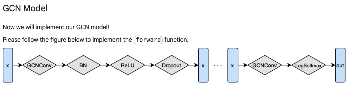
Feedforward Arichtectur

Weights are shared within GCN Layer but not across layers
- These weights are learned: “learn how to aggregate features of neighbors to optimize loss function”
Dropout sets certain features of output of layer to zero
BatchN rescales feature/embedding to more stable range (ca. mean = 0, variance = 1)
- done per feature dimension/ column wise across all nodes since we input a feature matrix
Relu sets negative feature/embebeding values to 0
Input of feedforward function is feature matrix and adjacency matrix

Learned weights:

Weight matrix in GCN layer
BatchNorm Parameters: scaling factor, shifting factor that applies after normalization

Graph classification

Same as node classification but loss is computed over $z_g$ graph level embeddings. Just using the forward passing in a GNN without training weights, we see a strong inductive bias: nodes that are close to each other have a similar embedding.

To train model we need to define:

criterion = Loss function
optimizer = e.g. ADAM

Classifiyer like softmax or sigmoind or linear is already part of feedforwad pass

Steps:

Forward pass
Compute loss (based on trainig nodes)
Derive gradiends
Update parameters based on gradients (optimizer)
Calculate Training accuracy (training nodes) /Validation acc (whole graph)
Repeat for as many epochs as wished

Graph Mini-BAtching

In order to parallelize: we combine graphs into a sinlge disconnected graph data object

We use global pooling over the nodes to create graph level embeddings that can be used to predict properties of graphs
- we need an index that states which nodes are of which graph
Since we have adj matrix in message passing, disconnected embeddings don’t influence other embeddings.
- but learned weights (GCN layer weights, batchNorm, etc.) are shared across disconnected graphs

Training and Optimization of GNN

Graph-level implementations

to make calculations more efficient graph level implementation of GNN equations are used.

$H^k = \sigma(AH^{(k-1)}W^k_{neigh} + H^{(k-1)}W_{self}^k)$ where $H^k$ is a matrix containing the layer-k embeedings of all nodes in the graph. We compute embedding $h_u^k$ exatctly once. Limitation one full batch gradient descent and memory problems.

==Subsampling and mini batching==

we can use standard regularization: L2, dropout, layer normalization

some GNN specific regularizations:

parameter sharing: use same parameters in all aggregate and update functions (most effective for GNN with more than 6 layers)
Edge dropout: randomly remove (or mask) edgeds in adjacency matrix during training

Computation graph

node’s neighborhood defines a computation graph
nodes aggregate information form their neighbors using neural networks
every node defines a computation graph based on its neighborhood
so that information of node v doesn’t get lost we include $h_v^{(l-1)}$

Computational Graph

Computational Graph

==Attention scores==

GNN layer in practice

Batch Normalization: stabilizes neural network training

Given a batch of inputs (node embeddings):

for each batch:

re-center the node emebeddings into zero mean
re-scale the variance into unit variance
apply trainable parameters to normalized feature input: $Y_{i,j} = \gamma X + \beta$

Dropout

Prevent overfitting:

during trainnig with some probability p, randomly set neurons to zero (turn off)
during testing use all the neurons for computation
in GNN it is applied in the linear layer in the message function

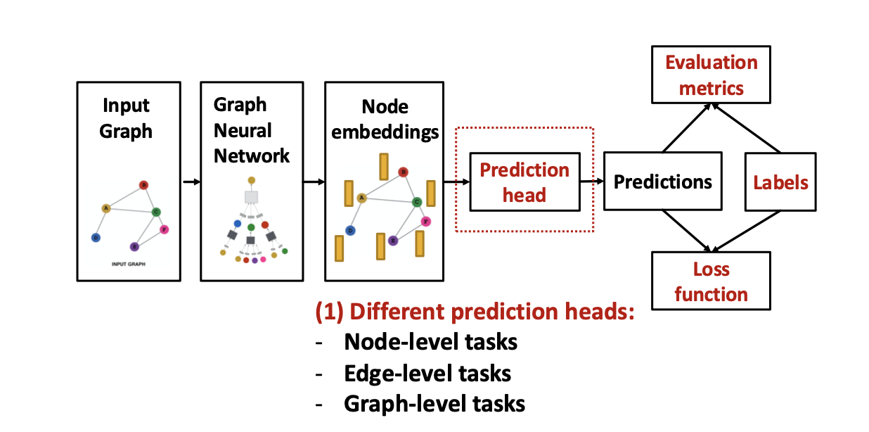
Training Pipeline

GNN Pipeline

GNN Pipeline

Different Tasks require different prediction heads:

Node-level prediction: directly make prediction using node embeddings. Classification and Regression
Edge-level-prediction: prediction using paris of node emebeddings.
- Options are: Concatenation + Linear $\hat y_{uv} = Linear(Concat(h_u,h_v))$
- Or: Dot product $\hat y_{uv} = (h_u)^Th_v$ $y^_{uv} = (h_{u})^{T} h_{v}$
  - only 1-way prediction (existence of an edge). Can be addapted to k-way prediction using trainable weights for each K
Graph-level prediction: prediction using all node embeddings
- Options are:
  - Global mean pooling, global max pooling, global sum pooling

Unsupervised signals on graphs Page 56

Evaluation metrics

Root mean square error (RMSE)
Mean absolute error (MAE)
Multi-class classification: accuracy (korrekt/total)
binary classification: accuracy, precision/recall, ROC AUC, F1

Page 66

Data Split

Fixed: split once

training: optimize GNN parameters
validation: develop model/hyperparameters
test: held out, test for final performance

Random: randomly split and report average across multiple random seeds

In graph we have problem that nodes are not independent, how to split?

Solution 1: Transductive setting

compute embeddings using entire graphs
train (compute loss) using node labels of 1/3 of nodes
validation node labels of second third
tes with last nodes

Solution 2: Inductive setting

break edges and split into multiple disconnected graphs

s74 # Exercise Wednesday

NLP Task

Lemmitization: reduce word to its base form (e.g. “running” to “run”) is important because it helps to reduce the dimensionality of the data and improve the performance of NLP models. By converting words to their base form, we can group together different forms of the same word (e.g., “run”, “running”, “ran”) and treat them as a single entity. This can help to improve the accuracy of tasks such as text classification, sentiment analysis, and information retrieval by reducing the sparsity of the data and allowing the model to learn more general patterns.
TF-IDF (Term Frequency-Inverse Document Frequency) is a numerical statistic that reflects the importance of a word in a document relative to a collection of documents (corpus). Term frequency (TF) of a word in a document by the inverse document frequency (IDF) of the word across the corpus.
- word appears often within a text but not across the corpus

Structure of data:

Modules: 222
- features: 25
Edge: prerequisites or dependencies (two types)
- ingoing: source mentioned in target module “Vorausgesetzte Kompetenzen”
- outgoing described in source module as “ergönzende und Vertiefende Module”

So two inconming edges have different types:

this is not reflected in the in-degree statistic

Unbalanced edge types

leads to favoring one type of edge over the other since loss is opimized for majority class

GraphSAGE

graph sample and aggregation

samples neighbors during message passing - doesn’t use all neighbors
effienct and better generalization
the dependency graph expands in classical gcn this can cause problems with mini-batching
oversmoothing problem with a lot of layers

Bayesian Networks and Causal Graphs

Simple statistics and AI can’t give us answers to causality questions.
Simposons Paradox is an example where different effects can be found in subpopulation compared to an average effect
Causal mechanism of the data generating process must be understood
Common causes (e.g. being a woman has effect on taking the drug and failure to recover) that effects both treatment and outcome is a confounder
common causes can cause spurious correlation

Causal story behind data

Structural causal model (SCM) - M

a way of describing relevant features of the world and how they interact with each other
edogenous: variables determined within the causal system
- part of causal mechanism
- influenced by other variables in the model
- is correlated with unobserved factors that affect outcome
- e.g. education/income
- caused by at least one exogenous variable
exogenous: variables that determined outside the causal system being modeled
- i.e. not caused by any variable inside the model
- not affected by other variables in the model
- often treated as independent inputs
- help identify causal effects because they provide variation that is not influenced by the outcome
- e.g.: completley randomly assigned scholarships

SCM consists of:

U: set of exogenous variables
V: set of endogenous variables
F: set of functions that assign each variable in V a value based on the values of the other variables in the model

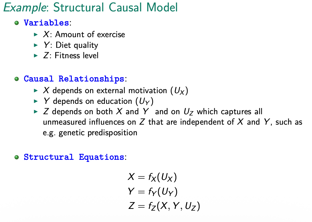
Graphical Causal Models

Every SCM is assocaited with a graphical causal model, and consists of:

set of nodes representing variables in U and V
set of edges representing the functions in f

edges can be directed vs. undirected
- starting node = parent
- end node = child
- for multiple connection: starting point == ancestor and every node on the path is descendant
Consequently, every endogenous variable in a model is a descendant of at least one exogenous variable
exogenous variables cannot be descendants of any other variables (root nodes in a graph).

Graphical definition of causation:

if in graphical model: X is child of Y then Y is direct cause of X. If x is desendant of Y, then Y is potential cause of X. ### DAG: Directed Acyclic Graphs (Bayesian networks)

to be Acyclic:

no self-lops or cycles

Explaining Away

Suppose we have two causes for an effect the conditional probability of one cause given effect is larger than conditional probaility of other cause given effect and second cause (even if both causes are independant)

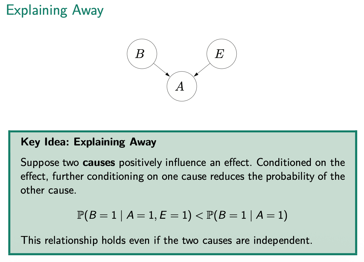- conditioning on A = 1 is crucial for explaining away phenomenon

Bayesian Network

Let $X=(X_1,...,X_n)$ be random variables. Bayesian network is a DAG that specifies a joint distribution over X as a product of local conditional distributions:

$\mathbb{P} = (X_1 =x_1,...X_n=x_n = \prod _{i=1}^np(x_i|x_{Parents(i)})$

if no direct connection in a DAG, then they nodes are conditional independent if connecting node is known:

$T \perp F|V$ which implies $p(f|v,t) = p(f|v)$

Causalality in Detail

Conditioning (Seeing) vs. Intervention (Doing) - Pearls Ladder of Causality

Conditioning: focuses on observed cases where a variable has a certain value ( $P(Y|X=x)$ ) - filters data - Intervention: forces a variable to take certain value, $P(Y|do(X=x)$ alters data-generating process

RCT = doing

with RCT we eliminate the connection between confouder and Treatment variable but the effect of confonder on Y stays Average Treatment Effect:

$ATE = \mathbb{E}[y|do(X=x_0)] - \mathbb{E}[Y|do(X=x_1)]$

Causal Conclusions form observational data

Target quantity is causal effect difference or average causal Effect (ACE)

$ACE = P(Y=1|do(X=1))- P(Y=1|do(X=0))$

Causal Machine Learning (GNN & Causal Graphs)

Oversvational setting:

$Y_i(1), Y_i(0) \perp W_i|X_i$

$Y_i(1)$ : potential outcome if unit i receives treatment
$Y_i(0)$ : potential outcome if unit i does not receive treatment
$W_i$ : treatment assignment for unit i
$X_i$ : observed covariates for unit i
After controlling for the observed covariates, the treatment assignment is as good as random, allowing us to estimate causal effects from observational data.
- unconfoundness

All sources of self-selection can be explained by observable covariates $X_i$

Propensity Scores

$e(X_I):= \mathbb{P}[W_i=1|X_i]$

in experiments usually known and fixed
in obersvational settings must be estimated

Overlap Assumption

$0 < e(X_i) < 1$ for all $X_i$

ensures that for every combination of covariates, there is a positive probability of receiving both treatment and control, allowing for meaningful comparisons between treated and untreated units across the range of covariates.

Difference-In-Means Estimator

common estimator of treament effect in exp. settings
sample average of outcomes in treatment minus control group:

Backdoor Criterion

do-operator (for example randomiztaion) erases arrows entering X.
backdoor criterion are variables that block every path between X and Y that contains an arrow into X & is no descendant of X
Parents of X always satisfies the backdoor criterion
do not condition on mediators
do not condition on colliders or their descendants (explaining away)
- if controlling/conditioning on collider know one cause can make unrelated causes appear related (spurious negative correlation)
- example talent -> Admission <- wealth: conditioning on admission (look only at admitted students)

collider

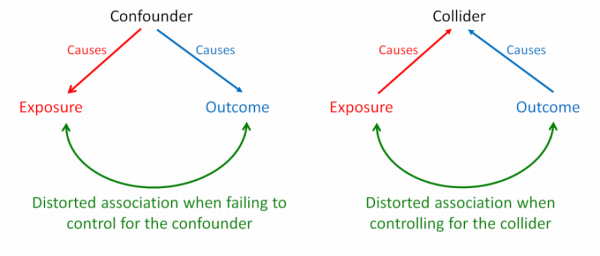
collider

Backdoor

Backdoor

This is a causal adjustment formular

What the true population effect looks like

If you analyze the entire population (without conditioning on heart disease):

Obesity increases mortality risk.
Smoking increases mortality risk.
No paradox.

The paradox appears only after conditioning on the collider.

Frontdoor Criterion

If there is a mediator M that lies on all causal paths from X to Y, and there are no unblocked backdoor paths from X to M or from M to Y, then the causal effect of X on Y can be identified using the front-door adjustment formula.

Adjustment Formular

The probability that 𝑌=𝑦if we intervene and set X =𝑥

The do(X=x) operator represents a forced intervention, like a randomized experiment.

Remove confounding is done by comparing people with same Z but different X. This is done by conditioning on Z. We calculate effect within each Z group and sum up the effects across all Z groups, weighted by the probability of each Z group occurring in the population. This allows us to estimate the causal effect of X on Y while controlling for the confounding variable Z.

P(Y=y|do(X=x)) = \sum_zP(Y=y|X=x,Z=z)P(Z=z)

Using conditional probabilites we can calculate the average causal effect (ACE):

P(Y=1|do(X=1)) - P(Y=1|do(X=0))

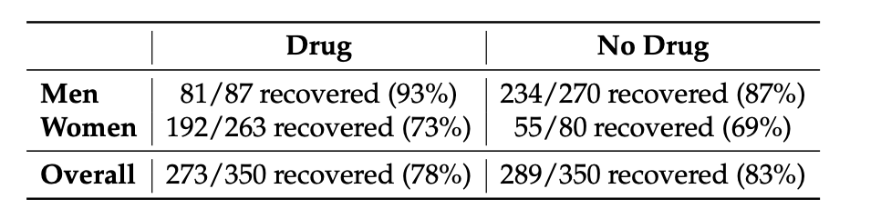
an ACT of 5% woudl mean: if everyone would take the drug 5% more people would recover compared to if no one would take the drug.

for continues z we use integrals instead of summation

Simpsons Paradox

Appears when a confounder affects both treatment assignment and outcome. A randomly selected subgroup of the population can show a different relationship between treatment and outcome than the overall population, leading to a paradoxical reversal of the observed effect when data is aggregated. If we randomly selected a patenint in treatment its most likely a women and women have less baseline recovery rate (generally less recovery due tue e.g. estrogen)