Simpson's paradox and mixed-effects models
How a trend can flip once you account for hierarchical structure, shown with the palmerpenguins data and random effects.
On this page
Simpson’s paradox is a statistical phenomenon that appears when data has a hierarchical structure. The data can be analysed at different levels of that structure, and the level you choose can change the result, and with it the answer to the research question. Simpson’s paradox is often used to show the advantages of linear mixed-effects models over simple linear regression.
Hierarchical data structures
Cross-sectional
Examples:
- Students nested in schools (two levels)
- Students nested in schools nested in cantons (three levels)
- Employees nested in companies (two levels)
Longitudinal
Examples:
- Exam grades nested in students (two levels)
- Customer satisfaction nested in people nested in age groups (three levels)
Example: penguins
Data (Gorman (2014)):
- palmerpenguins
- 344 penguins
- 3 species (Adélie, chinstrap and gentoo)
Dr Allison Horst, Alison Hill and Kristen Gorman turned the data into the R package palmerpenguins. This project is based on the tutorial by Silvia Canelon.
First, install the R packages
install.packages("palmerpenguins") #Data
install.packages("tibble") #Data handling
install.packges("ggplot2") #Plotting
install.packages("dplyr")
Load the packages
library(palmerpenguins)
library(tibble)
library(ggplot2)
library(dplyr)
penguins <- palmerpenguins::penguins
head(penguins)
# A tibble: 6 × 8
  species island    bill_length_mm bill_depth_mm flipper_length_mm body_mass_g
  <fct>   <fct>              <dbl>         <dbl>             <int>       <int>
1 Adelie  Torgersen           39.1          18.7               181        3750
2 Adelie  Torgersen           39.5          17.4               186        3800
3 Adelie  Torgersen           40.3          18                 195        3250
4 Adelie  Torgersen           NA            NA                  NA          NA
5 Adelie  Torgersen           36.7          19.3               193        3450
6 Adelie  Torgersen           39.3          20.6               190        3650
# ℹ 2 more variables: sex <fct>, year <int>
Explore the data
ggplot(data = penguins,
       aes(x = sex, y = body_mass_g))+
  geom_boxplot(aes(fill = species))
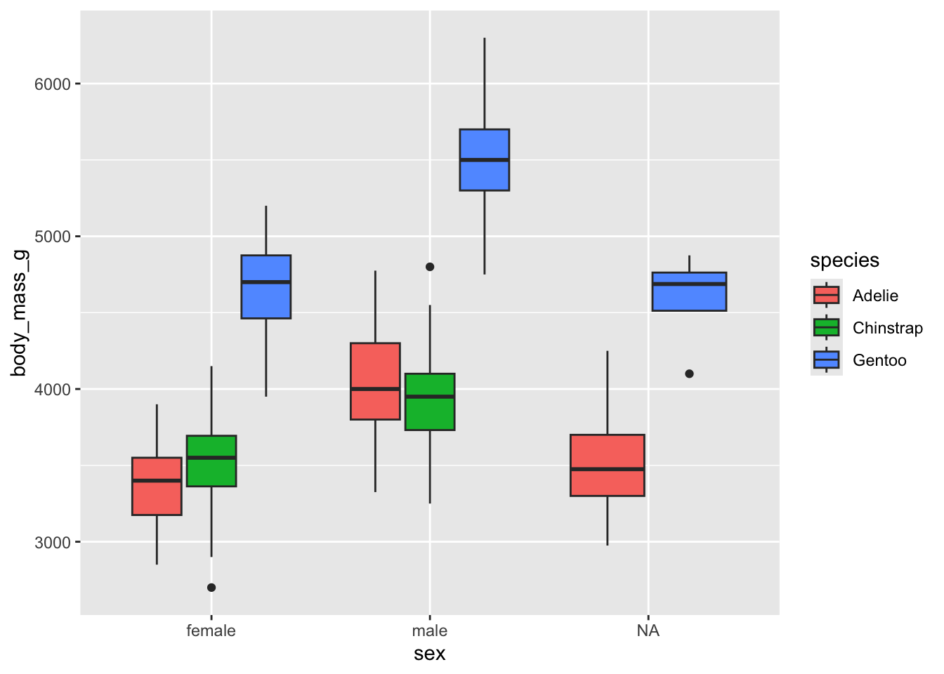
The box plots suggest a sex difference in body mass for gentoo penguins, which may not be the case for Adélie and chinstrap.
penguins %>%
  select(species, sex, body_mass_g) %>%
  arrange(desc(body_mass_g))
# A tibble: 344 × 3
   species sex   body_mass_g
   <fct>   <fct>       <int>
 1 Gentoo  male         6300
 2 Gentoo  male         6050
 3 Gentoo  male         6000
 4 Gentoo  male         6000
 5 Gentoo  male         5950
 6 Gentoo  male         5950
 7 Gentoo  male         5850
 8 Gentoo  male         5850
 9 Gentoo  male         5850
10 Gentoo  male         5800
# ℹ 334 more rows
penguins %>%
  select(species, sex, body_mass_g) %>%
  group_by(species,sex) %>%
  summarize(mean = mean(body_mass_g))
`summarise()` has grouped output by 'species'. You can override using the
`.groups` argument.
# A tibble: 8 × 3
# Groups:   species [3]
  species   sex     mean
  <fct>     <fct>  <dbl>
1 Adelie    female 3369.
2 Adelie    male   4043.
3 Adelie    <NA>     NA
4 Chinstrap female 3527.
5 Chinstrap male   3939.
6 Gentoo    female 4680.
7 Gentoo    male   5485.
8 Gentoo    <NA>     NA
penguins %>%
  group_by(species) %>%
  mutate(n_species = n()) %>%
  ungroup() %>%
  group_by(species,sex,n_species) %>%
  summarize(n=n())
`summarise()` has grouped output by 'species', 'sex'. You can override using
the `.groups` argument.
# A tibble: 8 × 4
# Groups:   species, sex [8]
  species   sex    n_species     n
  <fct>     <fct>      <int> <int>
1 Adelie    female       152    73
2 Adelie    male         152    73
3 Adelie    <NA>         152     6
4 Chinstrap female        68    34
5 Chinstrap male          68    34
6 Gentoo    female       124    58
7 Gentoo    male         124    61
8 Gentoo    <NA>         124     5
penguins %>%
  count(species, sex) %>%
  add_count(species, wt = n,
            name = "n_species")
# A tibble: 8 × 4
  species   sex        n n_species
  <fct>     <fct>  <int>     <int>
1 Adelie    female    73       152
2 Adelie    male      73       152
3 Adelie    <NA>       6       152
4 Chinstrap female    34        68
5 Chinstrap male      34        68
6 Gentoo    female    58       124
7 Gentoo    male      61       124
8 Gentoo    <NA>       5       124
penguins %>%
  count(species, sex) %>%
  add_count(species, wt = n,
            name = "n_species") %>%
  mutate(prop = n/n_species*100)
# A tibble: 8 × 5
  species   sex        n n_species  prop
  <fct>     <fct>  <int>     <int> <dbl>
1 Adelie    female    73       152 48.0
2 Adelie    male      73       152 48.0
3 Adelie    <NA>       6       152  3.95
4 Chinstrap female    34        68 50
5 Chinstrap male      34        68 50
6 Gentoo    female    58       124 46.8
7 Gentoo    male      61       124 49.2
8 Gentoo    <NA>       5       124  4.03
penguins %>%
  count(species, sex) %>%
  add_count(species, wt = n,
            name = "n_species") %>%
  mutate(prop = n/n_species*100) %>%
  filter(species == "Chinstrap")
# A tibble: 2 × 5
  species   sex        n n_species  prop
  <fct>     <fct>  <int>     <int> <dbl>
1 Chinstrap female    34        68    50
2 Chinstrap male      34        68    50
penguins_new <-
  penguins %>%
  mutate(year_factor = factor(year, levels = unique(year)))
penguins_new
# A tibble: 344 × 9
   species island    bill_length_mm bill_depth_mm flipper_length_mm body_mass_g
   <fct>   <fct>              <dbl>         <dbl>             <int>       <int>
 1 Adelie  Torgersen           39.1          18.7               181        3750
 2 Adelie  Torgersen           39.5          17.4               186        3800
 3 Adelie  Torgersen           40.3          18                 195        3250
 4 Adelie  Torgersen           NA            NA                  NA          NA
 5 Adelie  Torgersen           36.7          19.3               193        3450
 6 Adelie  Torgersen           39.3          20.6               190        3650
 7 Adelie  Torgersen           38.9          17.8               181        3625
 8 Adelie  Torgersen           39.2          19.6               195        4675
 9 Adelie  Torgersen           34.1          18.1               193        3475
10 Adelie  Torgersen           42            20.2               190        4250
# ℹ 334 more rows
# ℹ 3 more variables: sex <fct>, year <int>, year_factor <fct>
Visualize Simpson’s Paradox
ggplot(data = penguins,
       mapping = aes(x = bill_length_mm, y = bill_depth_mm))+
  geom_point() +
  geom_smooth(method='lm', formula = y ~x)
plot_simps <- penguins %>%
  ggplot(mapping = aes(x = bill_length_mm, y = bill_depth_mm, group = species, col = species)) +
  geom_point() +
  geom_smooth(method = 'lm', formula = y ~x)
plot_simps
Interpretation
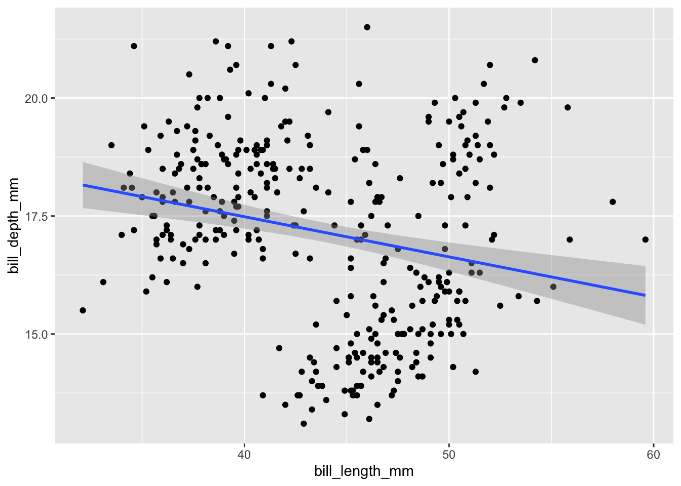
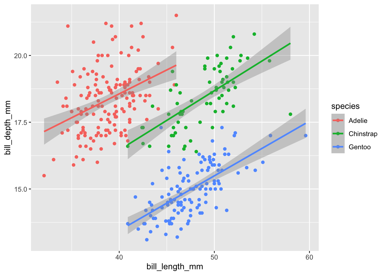
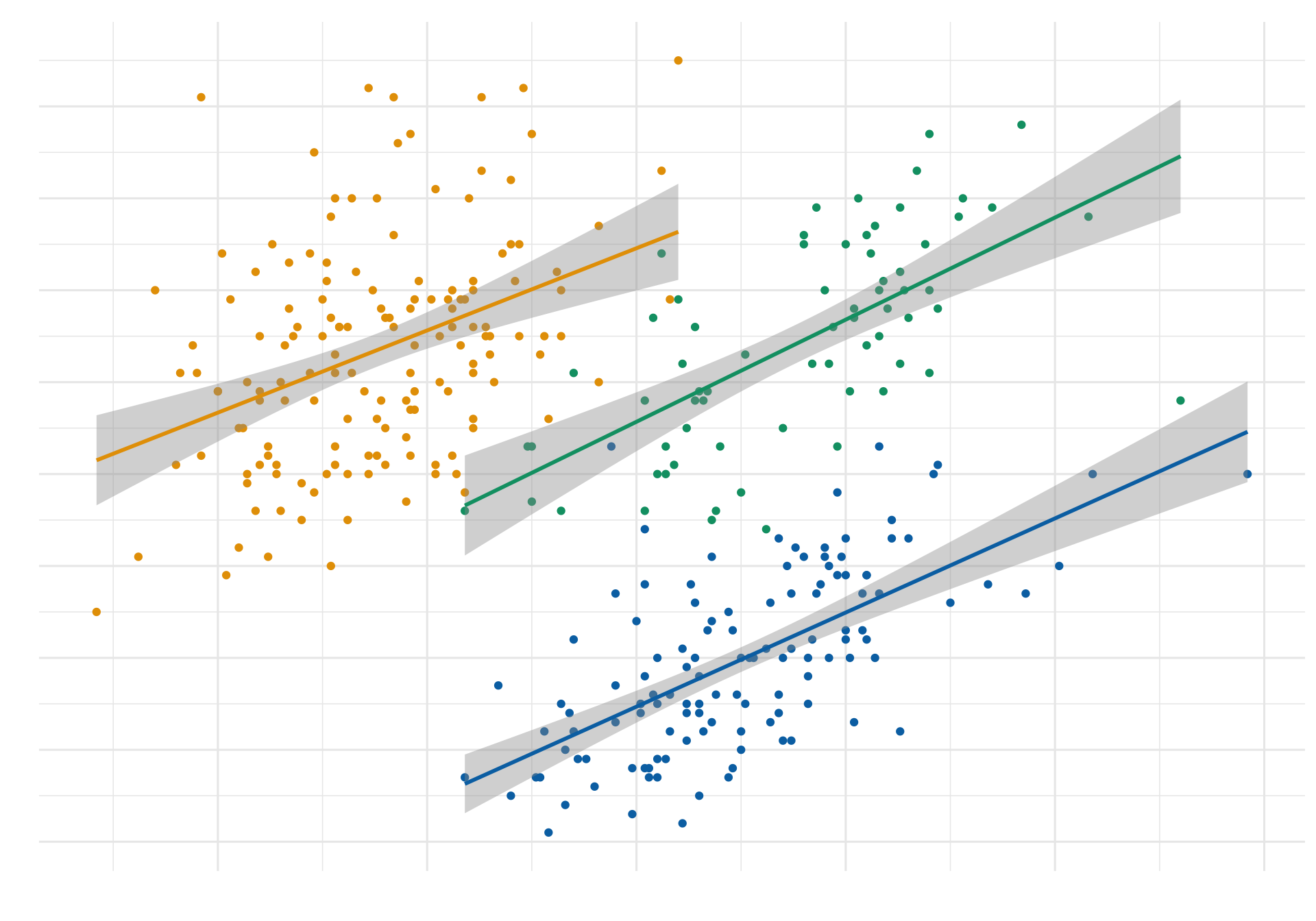
The last two plots show that if we ignore the penguins’ species, we draw the wrong conclusion about the relationship between bill length and bill depth.
More on mixed-effects models and Simpson’s paradox (see Hox, Moerbeek, and Van de Schoot 2017)
Let’s make a nice plot
Show code (29 lines)
library(thematic)
library(ggtext)
colors <- thematic::okabe_ito(3)
title_text <- glue::glue(
  'Bill Depth per Bill Length in mm for <span style = "color:{colors[1]}">**Adelie**</span>, <span style = "color:{colors[2]}">**Chinstrap**</span>, <span style = "color:{colors[3]}">**Gentoo**</span>')

plot_simps <- plot_simps  +
  labs(x = "Bill Lenght [mm]", y = "Bill Depth [mm]",
       color = "Species",
       title = title_text,
       caption = "Source: Penguins Data") +
  scale_y_continuous(
    breaks = 13:22
  )+
  scale_x_continuous(
    breaks = seq(30,60,by = 5)
    )+
  #guide = none, legend wird ausgelassen
  scale_color_manual(values = thematic::okabe_ito(3), guide = "none") +
  theme_minimal(base_family = 'Source Sans Pro', base_size = 12)+
  theme(plot.title = ggtext::element_markdown(color = 'grey20', size = rel(1.7),face= "bold"),
        plot.title.position = "plot",
  # Bold axis titles
  axis.title = element_text(face = "bold"),
  # Add some space above the x-axis title and make it left-aligned
  axis.title.x = element_text(margin = margin(t = 10), hjust = 0),
  # Add some space to the right of the y-axis title and make it top-aligned
  axis.title.y = element_text(margin = margin(r = 10), hjust = 1, margin (0,4,0,0)),)
plot_simps
Save plot
library(here)
here() starts at /Users/oliverzingg/Portfolio
p <- here("my_plot.png")
#ggsave(p,plot_simps, width=45, height=30, units = "cm", dpi=500)
Back to top
References
Gorman, Tony D. AND Fraser, Kristen B. AND Williams. 2014. “Ecological Sexual Dimorphism and Environmental Variability Within a Community of Antarctic Penguins (Genus Pygoscelis).” PLOS ONE 9 (March). https://doi.org/10.1371/journal.pone.0090081.
Hox, Joop J., Mirjam Moerbeek, and Rens Van de Schoot. 2017. Multilevel Analysis: Techniques and Applications. Routledge.