Generalized linear models

Depending on the outcome variable, we can use different types of models. For example, if the outcome variable is binary, we can use a logistic regression model. If the outcome variable is continuous, we can use a linear regression model. If the outcome variable is count data, we can use a Poisson regression model.

Binary and binomial dependent variable

Binary and binomial data naturally fall within the range of 0 to 1 (and are mathematically the same: binary = total number of trials is 1). Using a linear regression model would there predict values outside of this range. This would be a extrapolation which would make sense. Furthermore, in the case of logistic regression using a identity link function (i.e. linear regression) the predicted values would be heavily be influences by extreme values. Therefore, we adapt the linear regression based on attributes of the dependent variables. Additionally, we can’t assume normal distribution of errors for inference. Therefore, with this kind of data we assume other distributions as binomial distribution.

For binary and binomial data we use a logit link function that bounds the y between 0 and 1. The logit link function is defined as:

$$logit(y) = log(\frac{y}{1-y})$$

We therefore model the logit of y. The model transforms probabilities into log-odds so we can use linear modeling

$$logit(\text{probability of success: p}) = log(\frac{p}{1-p}) = \beta_0 + x_1*\beta_1...$$ $$exp(log(\frac{p}{1-p})) = \frac{p}{1-p} = exp(\beta_0) + exp(\beta_1)$$

For binomial data we use cbind(), for logistic regression we don’t use cbind().

glm.model <- glm(cbind("nr_of_successes", "nr_of_failures") ~ "predictor1" + "predictor2",
                 data = "data",
                 family = "binomial")

Multinomial dependent variable

Is a categorical variable with more than two levels. For example, the outcome variable could be a categorical variable with three levels: “low”, “medium”, and “high”. In this case, we can use a multinomial logistic regression model. The multinomial logistic regression model is an extension of the binary logistic regression model that allows for more than two categories. The multinomial logistic regression model uses a softmax function to model the probabilities of each category. The softmax function converts a vector of raw scores (logits) into a probability distribution, ensuring the sum of probabilities for all classes equals one.

library(nnet)
multinom.model <- multinom("outcome_variable" ~ "predictor1" + "predictor2",
                             data = "data")

Set cutoff

For logistic regression we set a cutoff the classify the outcome variable. The cutoff is the probability threshold above which we classify the outcome variable as 1 (success) and below which we classify the outcome variable as 0 (failure). The default cutoff is 0.5, but we can set a different cutoff based on the specific problem and the cost of false positives and false negatives.

glm.log <- glm("outcome_variable" ~ "predictor1" + "predictor2",
                 data = "data",
                 family = "binomial")
classification <- ifelse(fitted(glm.log) > 0.5, 1, 0)

Now let’s compare fitted vs. observed (confusion matrix)

compare <- data.frame(obs = df$obs,
                      fitted = classification)
# absolute
table(obs = compare$obs,
      fitted = compare$fitted)
# percentage
table(obs = compare$obs,
      fitted = compare$fitted) %>%
  prop.table() %>%
  round(digits = 2)

Naturally we would continue analysing different cutoff points with ROC and AUC.

Poisson regression

This model handels count data which is often encountered in real life situations where y data doens’t follow a normal distribution. Using a Linear model to model count data can lead to following problems:

• The predicted values can be negative, which is not possible for count data.
• The predicted values are not integers, which is also not possible for count data.
• The variance of count data naturally increases with the expected value (i.e. mean)

Idea

Change the linear model formular so that we only predict positive values:

$$\hat y = exp(\hat \beta_0 + \hat \beta_1*x_1)$$

this is equal to:

$$log(\hat y) = \hat \beta_0 + \hat \beta_1*x_1$$

We see that we can use natural logarithm as a link function. Next, we want y to be integer values and that the variance is dependent on the mean. Therefore, we use a Poisson distribution. The Poisson distribution is a discrete probability distribution that describes the number of events occurring in a fixed interval of time or space, given a known average rate of occurrence. The Poisson distribution is characterized by its mean (λ), which is also equal to its variance.

glm.poisson <- glm("outcome_variable" ~ "predictor1" + "predictor2",
                     data = "data",
                     family = "poisson")

Overdispersion

Dispersion parameter for poisson family taken to be 1 refers to the assumption that the variance increases linearly with the mean. In real life situations this is not the case. The variance is often larger than the mean. This is called overdispersion. In this case we can use a quasipoisson model.

Compare Residual deviance with the degrees of freedom. If the residual deviance is larger than the degrees of freedom, then we have overdispersion.

glm.poisson <- glm("outcome_variable" ~ "predictor1" + "predictor2",
                     data = "data",
                     family = "quasipoisson")

This imokies that the variance increases faster than linearly. The estimated coefficents are identifical but the standard error change and as a consequences the p-values change. ## GAM Extension of Linear Model to non-linearity

Interpretation of Coefficients

Poisson Model

#install.packages("faraway")
library(faraway)
library(tidyverse)

── Attaching core tidyverse packages ──────────────────────── tidyverse 2.0.0 ──
✔ dplyr     1.1.4     ✔ readr     2.1.5
✔ forcats   1.0.0     ✔ stringr   1.5.1
✔ ggplot2   3.5.1     ✔ tibble    3.2.1
✔ lubridate 1.9.4     ✔ tidyr     1.3.1
✔ purrr     1.0.2
── Conflicts ────────────────────────────────────────── tidyverse_conflicts() ──
✖ dplyr::filter() masks stats::filter()
✖ dplyr::lag()    masks stats::lag()
ℹ Use the conflicted package (<http://conflicted.r-lib.org/>) to force all conflicts to become errors

glm.complaints <- glm(complaints ~ . , data = esdcomp,
                      family = "poisson")

summary(glm.complaints)

Call:
glm(formula = complaints ~ ., family = "poisson", data = esdcomp)

Coefficients:
              Estimate Std. Error z value Pr(>|z|)
(Intercept) -0.0803448  1.1542122  -0.070  0.94450
visits       0.0009499  0.0003386   2.806  0.00502 **
residencyY  -0.2319740  0.2029388  -1.143  0.25301
genderM      0.1122391  0.2235043   0.502  0.61554
revenue     -0.0033827  0.0041553  -0.814  0.41560
hours       -0.0001569  0.0006634  -0.237  0.81298
---
Signif. codes:  0 '***' 0.001 '**' 0.01 '*' 0.05 '.' 0.1 ' ' 1

(Dispersion parameter for poisson family taken to be 1)

    Null deviance: 89.447  on 43  degrees of freedom
Residual deviance: 49.995  on 38  degrees of freedom
AIC: 184.77

Number of Fisher Scoring iterations: 5

Since we are modelling log(y) we have to exponentiate (inverse functions) the coefficients to get the multiplicative effect of a one unit increase in the predictor variable on the expected value of y.

Factor

exp(coef(glm.complaints)["genderM"]) %>% round(digits = 2)

genderM
   1.12

Continous

exp(coef(glm.complaints)["visits"]) %>% round(digits = 5)

 visits
1.00095

Increase in visist by one is not really interesting:

range(esdcomp$visits)

[1]  879 3763

exp(coef(glm.complaints)["visits"]*50) %>% round(digits = 5)

 visits
1.04864

Binomial Model

glm.insects <- glm(cbind(dead, alive)~ conc,
                  family = "binomial",
                  data = bliss)

summary(glm.insects)

Call:
glm(formula = cbind(dead, alive) ~ conc, family = "binomial",
    data = bliss)

Coefficients:
            Estimate Std. Error z value Pr(>|z|)
(Intercept)  -2.3238     0.4179  -5.561 2.69e-08 ***
conc          1.1619     0.1814   6.405 1.51e-10 ***
---
Signif. codes:  0 '***' 0.001 '**' 0.01 '*' 0.05 '.' 0.1 ' ' 1

(Dispersion parameter for binomial family taken to be 1)

    Null deviance: 64.76327  on 4  degrees of freedom
Residual deviance:  0.37875  on 3  degrees of freedom
AIC: 20.854

Number of Fisher Scoring iterations: 4

Continous

exp(coef(glm.insects)["conc"]) %>% round(digits = 2)

conc
 3.2

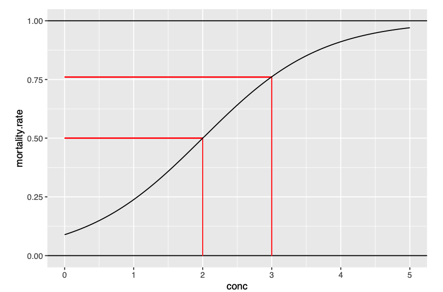
Odds of our model

With one unit increase in concentration, the odds of death increase by a factor of 3. This means that the odds of death are 3 times higher for each unit increase in concentration:

$$1:\frac{1}{3} \rightarrow 1:1 \rightarrow 1:3$$

Factors

Divide by 4

Quick interpretation of odds as upper bound increase in probability of y = 1.

Overdispersion

You can add quasibinomial to the family argument. This will give you a dispersion parameter that is greater than 1. But only works for binomial data and not binary.

Back to top