Orthonormal bases

Used in matrix multiplication. For two vectors use 1D array in python

import numpy as np
v = np.array([[1],[2],[3]])
g = np.array([[3],[2],[1]])

print((v.T@g)[0,0])
#or
print(np.dot(v.T,g)[0,0])

Definition:

Show code (13 lines)

$$\mathbf{x} \bullet \mathbf{y} = \begin{bmatrix} x_1 \\ \vdots \\ x_n \end{bmatrix} \bullet \begin{bmatrix} y_1 \\ \vdots \\ y_n \end{bmatrix} = x_1 y_1 + \cdots + x_n y_n = \sum_{i=1}^n x_i y_i$$

Exercise 6.1.

Norm

Euclidean Norm is has a geometrical interpretation. Using pythagorean theorem as often as $\mathbb{R}^2-1$ we get the norm or length of a vector

$$\|x\| = \left\| \begin{bmatrix} x_1 \\ x_2 \\ \vdots \\ x_n \end{bmatrix} \right\| = \sqrt{x_1^2 + \cdots + x_n^2}$$

Linearity of the Euclidean norm doesn’t hold:

$$\left\|x + y \right\| \not= \left\|x\right\|+ \left\|y\right\|$$

In fact:

$$\left\|x + y \right\| < \left\|x\right\|+ \left\|y\right\|$$

Since geometrically x+y represents the fast way (Triangle inequality).

The dot product of a vector with itself is the squared Euclidean norm:

$$x \bullet x = \left\| x\right\|^2$$

Manhattan norm

Defined by: $\left\| x \right\|_1 = |x_1|+\cdots+|x_n|$

Norm

Metric

Orthogonal Projection

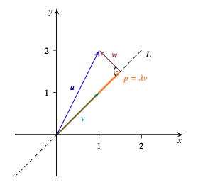Orthogonal Projection onto a line spanned by vector v.

$$projection = \frac{u \bullet v}{\left\|v\right\|^2}*v$$

Find orthogonal vector w:

$$w = u-p$$

we can write w as $u = p + w$ and yields a decomposition of u as sum of two vectors which are orthogonal.

Orthonormal

A set is orthogonal if any two vectors in that set are orthogonal (i.e., linear independent: $dot \space product = 0$ or $u\bullet v = 0$).

A set is orthonormal if any two vectors in that set are orthogonal and each vector is normalized (i.e., $norm = 1$ or $u\bullet u = 1^2$).

• An orthonormal set is also called orthonormal system (ONS for short).
• Normalize vectors by diving each components with the norm ($\left\|vector\right\|$) of vector.
• Orthonormal basis span a vector space:
  • each vector $v$ in that space can be formulated as linear transformation of those basis $b_1,b_2$.
  • Finding the coordinates $a_1,a_2$ can be done by $a_1 = v\bullet b_1$ and $a_2=v \bullet b_2$.

$$v = (v\bullet b_1)*b_1 + (v\bullet b_2)*b_2$$

Whats the use of orthonormal basis (ONB)?

U linear subspace of $\mathbb{R}^2$ and $b_1,...b_k$ is orthonormal basis of U. Then, for each $vector \in U$ we have:

$$vector = a_1*b_1 +a_2*b_2 +...a_k*b_k$$

so we can decompose each vector into a linear combination of the orthonormal basis (think in geometrical terms where we scale and add x and y basis to display a vector). $a_1,..$ are the coordinates with respect to the basis and we normally have to solve a linear system with gaussian elimination to find these coordinates (where coordinates are the unknown: $s_1,s_2,..$).

But with ONB we can directly calculate these coordinates with dot product:

$$vector = (v\bullet b_1)b1 + ...$$

In $\mathbb{R}^2$ with $î$ and $\hat j$:

$$[5 \space 6] = ([5 \space 6]^t \bullet [1 \space 0]^t) * [1 \space 0]^t+ ([5\space 6]^t \bullet [0 \space 1]^t) * [0 \space 1]^t$$

The coordinate vector of $[5 \space 6]$ is $[5 \space 6]$ with respect to basis $i$ and $j$ but these are normally not the same.

Gram-Schmidt Process

Tips for normalizing (extract annoying variables that get canceld out later here $\pi$ ):

$$\left\|\begin{pmatrix} \frac{6}{\pi} \\ \frac{-7}{\pi} \\ \frac{-6}{\pi}\end{pmatrix} \right\| = \frac{\frac{1}{\pi} \begin{pmatrix} 6 \\ -7 \\ -6\end{pmatrix}}{\frac{1}{\pi}\left\|\begin{pmatrix} 6 \\ -7 \\ -6\end{pmatrix}\right\|} = \frac{1}{\sqrt{6^2+(-7)^2+(-6)^2}}\begin{pmatrix} 6 \\ -7 \\ -6\end{pmatrix}$$

Python:

numpy.linalg.norm(v,1) #Manhattan-norm
numpy.linalg.norm(v,2) #Euclidean-norm Deafault
numpy.linalg.norm(v,np.inf) #Maxnorm

# Gram-Schmidt-Process

Q,R = numpy.linalg.qr(A) #retursn two matrices: Q is results, R additional Infos

Spectral Theorem

Facts about: symmetric matrices (A = A.T)

• Must be square matrix ($n * n = \mathbb{R}^n$)
• Diagonalizable (so there exist an eigenbasis of $\mathbb{R}^n$: so we can transfrom A with matrix consisting of eigenbasis)
• if eigenvectors are different -> eigenspaces of these vectors are orthogonal
  • decomposed original space into subspaces which are orthogonal
• Applying Gram-Schmidt on all eigenspaces, one obtains an orthonormal basis consisting of eigenvectors of A$ ^n$

Facts about: Orthogonal Matrices:

• if $v_1,..v_n \in \mathbb{R}^n$ and form ONB:
  • Then the matrix V consisting of $v_1,..v_n$ satisfies: $V^TV=I_n$ since dot product of individual columns are zero except with itself (gives 1).
• Matrix V is called orthogonal (better: orthonormal?)
• Inverse of V is $V^T$ -Finally: $V^TAV=diagonale(A)$
• Principal Axis Transformation(Matrix decomposition) $ A = VDV^T$

How to calculate V?:

• Find all eigenvectors(+values)
• Apply Gram-Schmidt to all eigenspaces

Singular Value Decomposition (SVD)

“Generalization of eigenvalue decomposition”. SVD exists for all matrices not just squared ones.

Principale Axis Decomposition:

• A symmetric: $A = VDV^t$
  • $V$ is orthogonal, $D$ diagonale
  • If A symmetric then SVD is the same.
• A general (rectangle): $A= U\Sigma V^T$
  • $U$ orthogonal, $\Sigma$ orthogonal(“diagonal”)

$\Sigma$ has same shape as A with $\sigma_1,..\sigma_n$ as diagonal entries everything else is zero. These entries are the singular values of A (generalization of eigenvalues). We are only interested in non-zero singular values which equals the rank of A.

Angles between vectors

Back to top