How sample size affects variable selection
A simulation of how often lm() and stepwise selection pick the true predictors as the sample grows.
Simulation20223 min readSimulationRegressionR

With this exercise we want to inspect how lm function and step function vary when it comes to selection of correct variables depending on sample size.
Foto von Jackson Jost auf Unsplash
Generate Data
Show code (113 lines)
# Load packages
library(lme4)
library(dplyr)
library(ggplot2)

options(scipen=0)
set.seed(101)

# Variable and Dataset preparation
N <- c(25, 30, 40, 60, 100 ,500, 1000)
# create a data frame to later add which variables were selected
predi_selection_lm <- as.data.frame(matrix(NA, nrow = 19, ncol = length(N)))
predi_selection_step <- as.data.frame(matrix(NA, nrow = 19, ncol = length(N)))

names(predi_selection_lm ) <- c("N25", "N30", "N40", "N60", "N100", "N500", "N1000")
names(predi_selection_step ) <- c("N25", "N30", "N40", "N60", "N100", "N500", "N1000")

#counter to use as index for table predi_selection (loop)
a = 1

#loop over different N (sample size)
for(i in N){
  # Simulation dataset
  x1 <- runif(i, 0, 10)
  x2 <- runif(i, 0, 10)
  x3 <- runif(i, 0, 10)
  x4 <- runif(i, 0, 10)
  x5 <- runif(i, 0, 10)
  x6 <- runif(i, 0, 10)
  x7 <- runif(i, 0, 10)
  x8 <- runif(i, 0, 10)
  x9 <- runif(i, 0, 10)
  x10 <- runif(i, 0, 10)
  x11 <- runif(i, 0, 10)
  x12 <- runif(i, 0, 10)
  x13 <- runif(i, 0, 10)
  x14 <- runif(i, 0, 10)
  x15 <- runif(i, 0, 10)
  x16 <- runif(i, 0, 10)
  x17 <- runif(i, 0, 10)
  x18 <- runif(i, 0, 10)
  x19 <- runif(i, 0, 10)
  err <- runif(i, 0, 5)

  data <- cbind(x1,x2,x3,x4,x5,x6, x7, x8, x9 ,x10, x11, x12, x13, x14, x15, x16, x17, x18, x19,  err)
  data <- as.data.frame(data)

  # generate y values.
  y <- 30 + 0.4*x1 + 1*x2 + 2.3*x3 + 0.7*x4 + 0.2*x5  + 1*x6 + 2*x7 + 3*x8 + 1.5 *x9 + 0.5*x10 + err

  # add generated y values to data frame
  data_2 <- cbind(data, y)

  # Modelling with all variables as predi.
  mod <- lm(y~ x1 + x2 + x3 + x4 + x5 + x5 +x6 + x7 + x8 + x9 + x10 + x11 + x12 + x13 + x14 + x15 + x16 + x17 + x18 + x19, data =  data_2)
  summary(mod)

  ########################
  #lets try step function#
  ########################


  # use step function and save final model as stepwise_model
  stepwise_model <-  step(mod)


  # Extract p-val: lm
  p_val_lm <- (summary(mod)$coefficients[,4])
  p_val_lm <- p_val_lm[2:20] #take out intercept

  # Extract p-val: step
  p_val_step <- summary(stepwise_model)$coefficients[,4]
  p_val_step <- p_val_step[2:20] #take out intercept

  # Store value: lm
  predi_selection_lm[a] <- ifelse(p_val_lm < 0.05, 1, 0)

  #store values for step different, because summary output dosen't include all variable like in lm
  p_val_step <-  na.omit(ifelse(p_val_step < 0.05, 1, 0))

   #remove selected pred. without 0.05
  p_val_step <- p_val_step[! p_val_step %in% 0]

  # save the names of all selected coefficients as coes
  coes <- names(p_val_step)

  # create dummy var with all possible variables
  dummy_var <- c('x1','x2','x3','x4','x5','x6','x7','x8','x9','x10','x11','x12','x13','x14','x15','x16','x17','x18','x19')

  # which out of all possible variable have been selected?
  selected_coe <- ifelse(dummy_var %in% coes, 1,0)

  predi_selection_step[a] <- selected_coe

  #increase counter by one
  a = a + 1
}

# Summary accuracy predictors selection
true_pred_dummy <- c(1,1,1,1,1,1,1,1,1,1,0,0,0,0,0,0,0,0,0) #dummy code for the existing predictor

# new data frame to compare true predi. to selected predi.
predi_accuracy_lm <- data.frame(matrix(NA, nrow = 19, ncol = length(N)))
names(predi_accuracy_lm) <- c("N25", "N30", "N40", "N60", "N100", "N500", "N1000")

predi_accuracy_step <- data.frame(matrix(NA, nrow = 19, ncol = length(N)))
names(predi_accuracy_step) <- c("N25", "N30", "N40", "N60", "N100", "N500", "N1000")

#if all correct than coloumn all 1.
for (j in 1:length(N)){
  predi_accuracy_lm[j] <- ifelse(predi_selection_lm[j] == true_pred_dummy, 1,0)
  predi_accuracy_step[j] <- ifelse(predi_selection_step[j] == true_pred_dummy, 1,0)
}
Now lets visualize these results
Show code (18 lines)
# final data frame used for visualization
sample_s <- c("N25", "N30", "N40", "N60", "N100", "N500", "N1000")
summary_accuracy <- data.frame(cbind(sample_s,rep(NA, times = length(sample_s)),rep(NA, times = length(sample_s))))
names(summary_accuracy) <- c("sample_s", "accuracy_lm", "accuracy_step")

for( i in 1: nrow(summary_accuracy)){
  summary_accuracy[i,2] <-  mean(predi_accuracy_lm[,i])
  summary_accuracy[i,3] <-  mean(predi_accuracy_step[,i])

}
summary_accuracy$accuracy_lm <- as.numeric(summary_accuracy$accuracy_lm)
summary_accuracy$accuracy_step <- as.numeric(summary_accuracy$accuracy_step)
ggplot(data = summary_accuracy,aes(x=factor(sample_s,
                                           level = c("N25", "N30", "N40", "N60", "N100", "N500", "N1000")) ,
                                            y = accuracy_lm)) +
  geom_bar(stat= "identity")+
  xlab("sample size")+
  labs(title = "Accuracy of selected predictor per sample size")
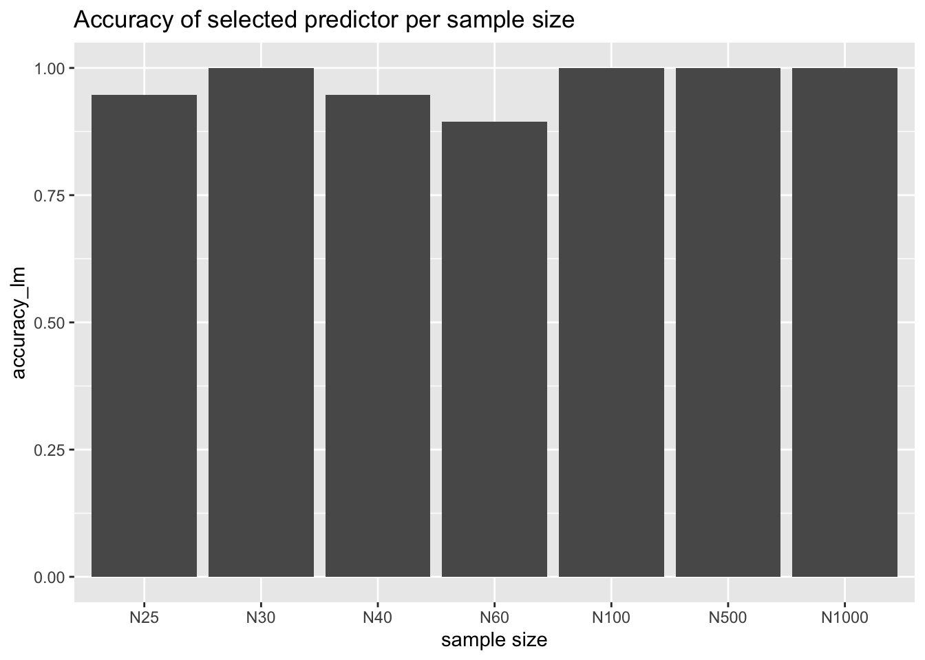
This is the accuracy of the normal lm function with all predictors used.
ggplot(data = summary_accuracy,aes(x=factor(sample_s,
                                           level = c("N25", "N30", "N40", "N60", "N100", "N500", "N1000")) ,
                                            y = accuracy_step)) +
  geom_bar(stat= "identity")+
  xlab("sample size")+
  labs(title = "Accuracy of selected predictor per sample size")
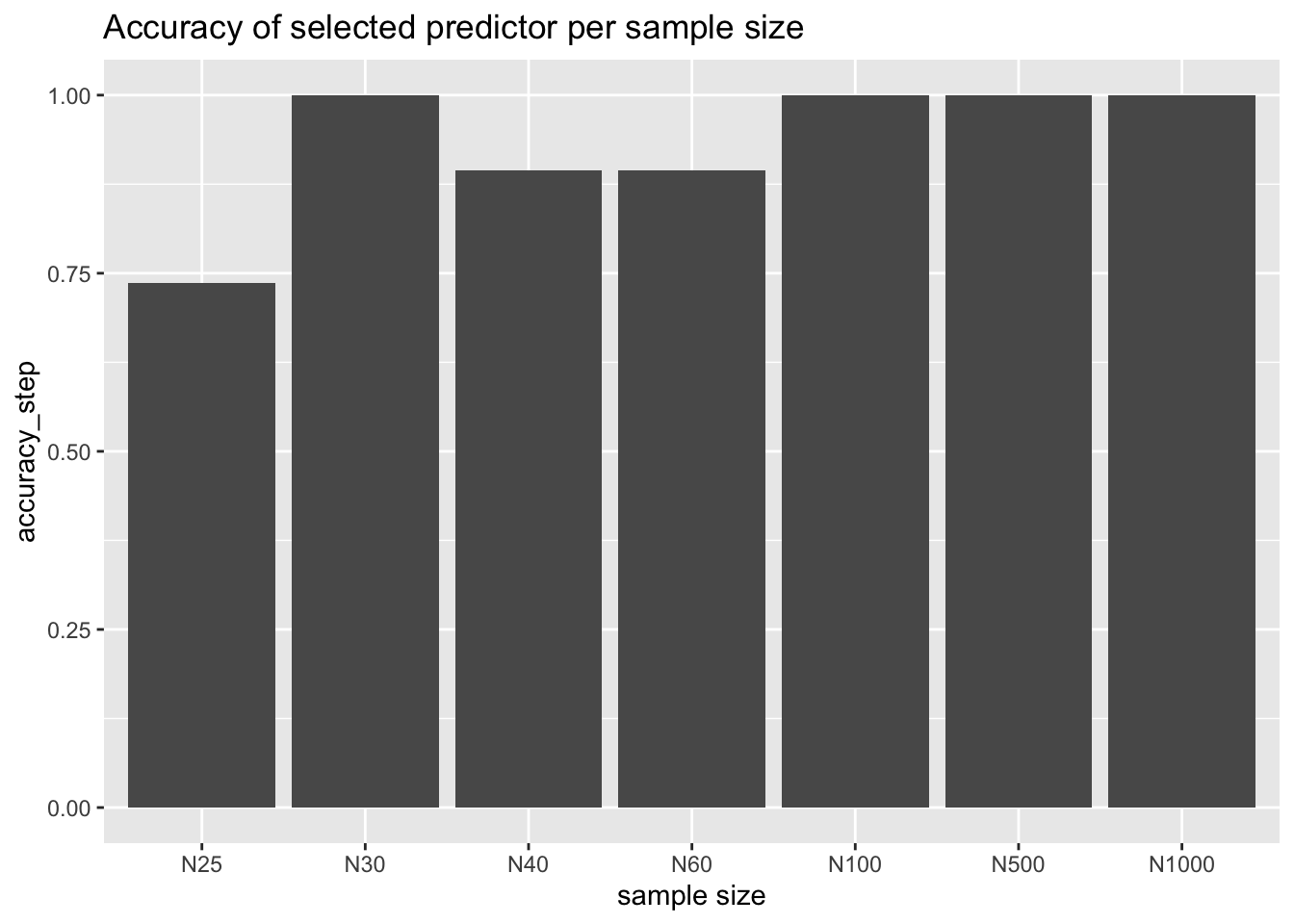
This is the accuracy of the step function default = backwards selection (starting with full model: all predictors) .
Summary:
- especially with low sample size N25 step function seems to perform less well than normal lm function
- with increasing sample size both perform well and use all relevant predictors
Back to top