Confidence intervals by simulation

Full credit goes to: https://www.kaggle.com/code/hamelg/intro-to-r-part-23-confidence-intervals/notebook
My contribution is only adding comments to learn from this code as much as possible
More on confidence intervals can be found here Hoekstra et al. (2014)

Generating data

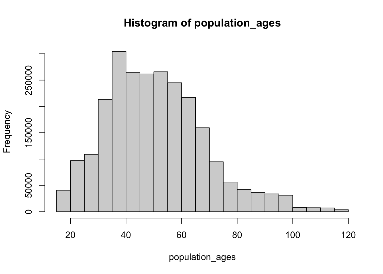
The following example simulates the process of finding the mean age value of a population of voters.

First we generate a population with their age values
- 1 Million values a generated from an exponential distribution and 1.5 Million values from a poisson distribution
- 18 is added to make sure that no age value is below 18 years old.
For numbers higher than 100 the modulo (%%) is taken and 18 is added to make sure we don’t end up with too large numbers.

set.seed(12)

# Generate a population
population_ages <- c(rexp(1000000,0.015)+18,
                    rpois(500000,20)+18,
                    rpois(500000,32.5)+18,
                    rpois(500000,45)+18)

population_ages <- ifelse(population_ages<100,
                          population_ages, population_ages%%100+18)

true_mean <- mean(population_ages)   # Check the population mean

true_mean

Drawing different sample from the population and calculating the mean

The central limit theorem states that the distribution of the mean values are normally distributed no matter what the distribution is of the population.

Let’s visualize the distribution of mean values. A skewness of 0 would be a normal distribution.

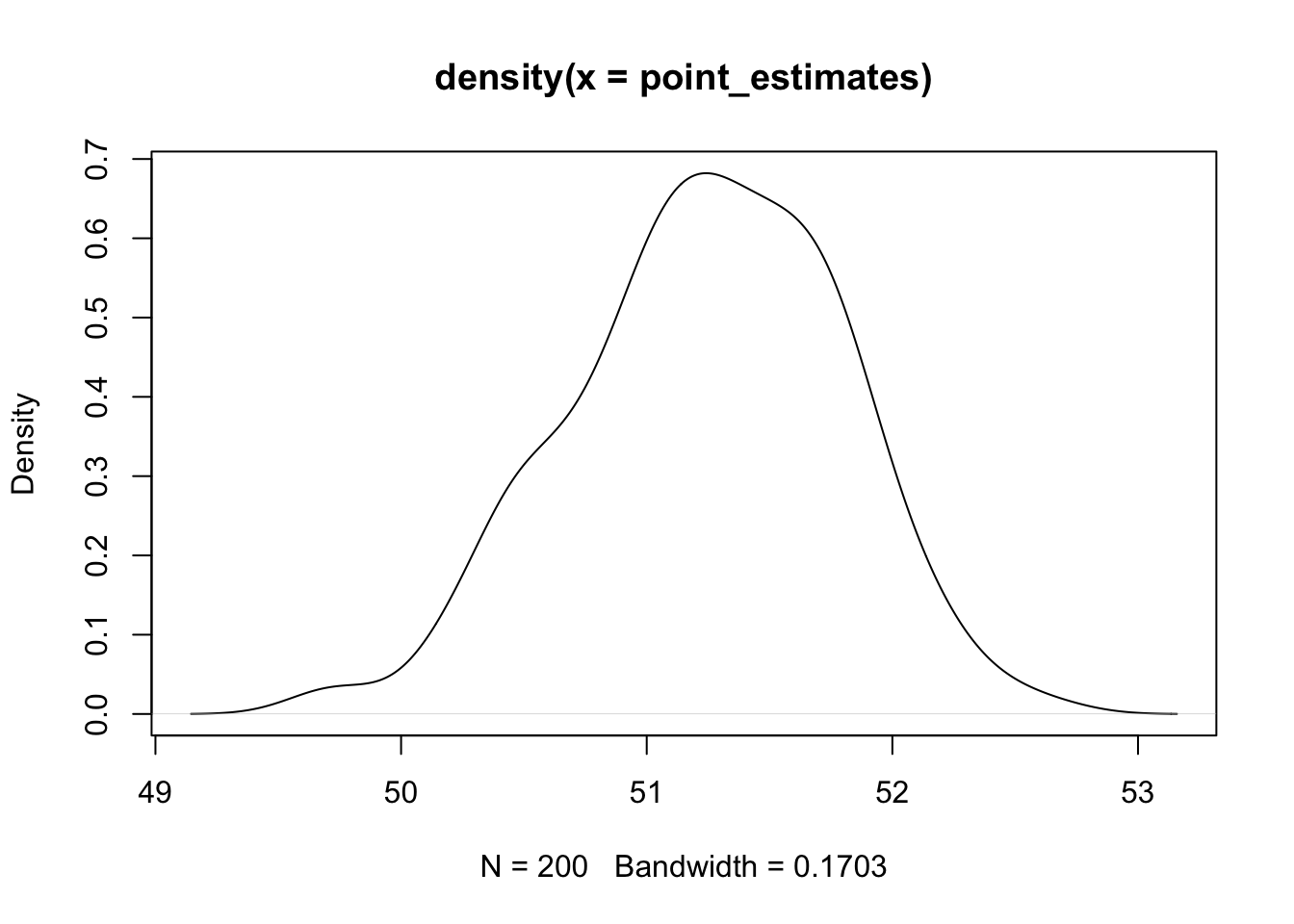
[1] -0.2609927

Confidence Intervals for the mean values

First the sample size is determined then an empty vector is created that will store the boundaries of all confidence intervals
The for loop is set to 25, meaning we draw a sample of size 1000 25 times.
With qnorm we can get the z value that is used to calculate the boundaries of the confidence intervals

Show code (23 lines)

set.seed(12)
sample_size <- 1000

intervals <- c()  # Create and store 25 intervals

for (sample in 1:25){
sample_ages <- sample(population_ages, size=sample_size)  # Take a sample of 1000 ages

sample_mean <- mean(sample_ages)  # Get the sample mean

z_critical <- qnorm(0.975)        # Get the z-critical value*

pop_stdev <- sd(population_ages)  # Get the population standard deviation

margin_of_error <- z_critical * (pop_stdev / sqrt(sample_size)) # Calculate margin of error

confidence_interval  <- c(sample_mean - margin_of_error,  # Calculate the the interval
                          sample_mean + margin_of_error)

intervals <- c(intervals, confidence_interval)
}

interval_df <- data.frame(t(matrix(intervals,2,25)))  # Store intervals as data frame

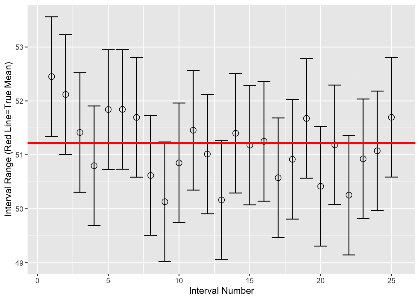
Plotting the 25 confidence intervals

The red line shows the true mean. We see the first confidence interval not including the true mean. (1/25 = 0.04)

Summary

Simulating confidence interval shows that some will not include the true value.

References

Hoekstra, Rink, Richard D. Morey, Jeffrey N. Rouder, and Eric-Jan Wagenmakers. 2014. “Robust Misinterpretation of Confidence Intervals.” Psychonomic Bulletin & Review 21 (5): 1157–64. https://doi.org/10.3758/s13423-013-0572-3.