Themes and annotations in ggplot2
Using themes and annotations to surface the story in a chart, with the gapminder data.
Visualisation20234 min readggplot2VisualisationR
On this page
Show code (23 lines)
library(tidyverse)  # For ggplot, dplyr, and friends
library(gapminder)  # For gapminder data
library(scales)     # For nice axis labels

gapminder_filtered <- gapminder %>%
  filter(year > 2000)

base_plot <- ggplot(data = gapminder_filtered,
                    mapping = aes(x = gdpPercap, y = lifeExp,
                                  color = continent, size = pop)) +
  geom_point() +
  # Use dollars, and get rid of the cents part (i.e. $300 instead of $300.00)
  scale_x_log10(labels = dollar_format(accuracy = 1)) +
  # Format with commas
  scale_size_continuous(labels = comma) +
  # Use viridis
  scale_color_viridis_d(option = "plasma", end = 0.9) +
  labs(x = "GDP per capita", y = "Life expectancy",
       color = "Continent", size = "Population",
       title = "Here's a cool title",
       subtitle = "And here's a neat subtitle",
       caption = "Source: The Gapminder Project") +
  facet_wrap(vars(year))
Create and save theme (my_pretty_theme)
Show code (23 lines)
my_pretty_theme <- theme_minimal(base_family = "Roboto Condensed", base_size = 12) +
  theme(panel.grid.minor = element_blank(),
        # Bold, bigger title
        plot.title = element_text(face = "bold", size = rel(1.7)),
        # Plain, slightly bigger subtitle that is grey
        plot.subtitle = element_text(face = "plain", size = rel(1.3), color = "grey70"),
        # Italic, smaller, grey caption that is left-aligned
        plot.caption = element_text(face = "italic", size = rel(0.7),
                                    color = "grey70", hjust = 0),
        # Bold legend titles
        legend.title = element_text(face = "bold"),
        # Bold, slightly larger facet titles that are left-aligned for the sake of repetition
        strip.text = element_text(face = "bold", size = rel(1.1), hjust = 0),
        # Bold axis titles
        axis.title = element_text(face = "bold"),
        # Add some space above the x-axis title and make it left-aligned
        axis.title.x = element_text(margin = margin(t = 10), hjust = 0),
        # Add some space to the right of the y-axis title and make it top-aligned
        axis.title.y = element_text(margin = margin(r = 10), hjust = 1),
        # Add a light grey background to the facet titles, with no borders
        strip.background = element_rect(fill = "grey90", color = NA),
        # Add a thin grey border around all the plots to tie in the facet titles
        panel.border = element_rect(color = "grey90", fill = NA))
base_plot +
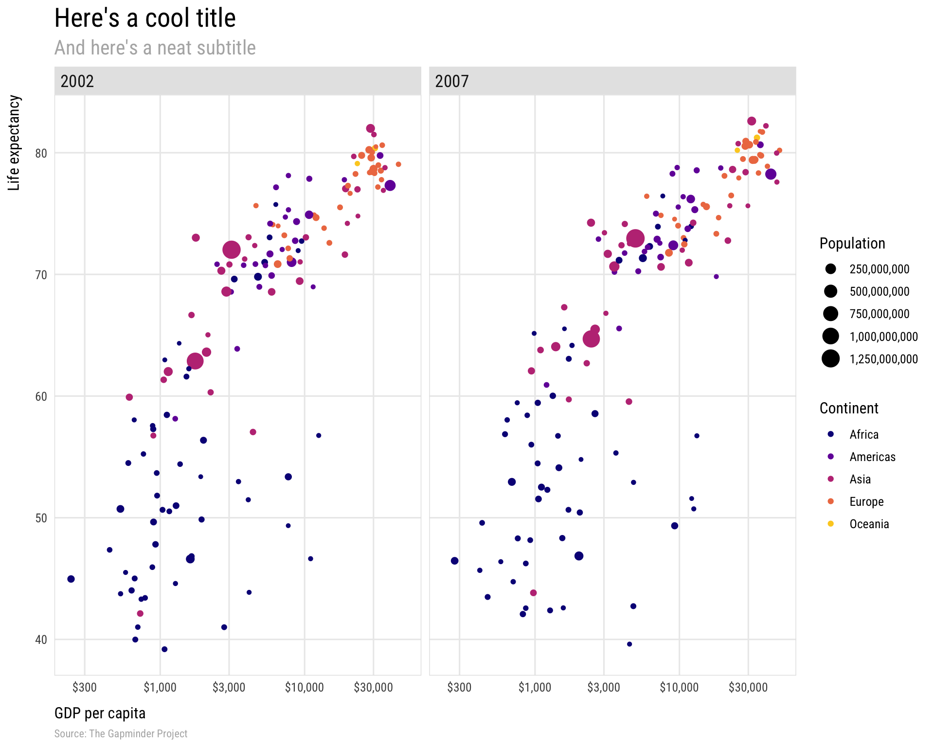
  my_pretty_theme
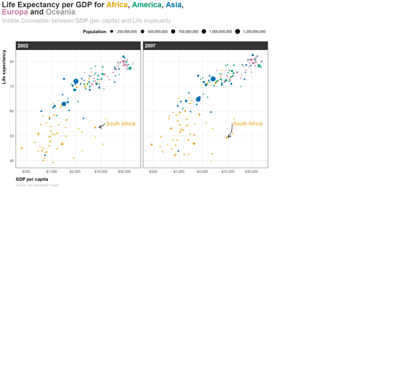
Lets make this plot even better :D
Show code (64 lines)
library(tidyverse)
library(gapminder)
library(scales)
library(ggtext)
library(thematic)

gapminder_filtered <- gapminder %>%
  filter(year > 2000)

colors <- thematic::okabe_ito(5)
title_text <- glue::glue(
  ' Life Expectancy per GDP for <span style = "color:{colors[1]}">**Africa**</span>, <span style = "color:{colors[2]}">**America**</span>, <span style = "color:{colors[3]}">**Asia**</span>, <br> <span style = "color:{colors[4]}">**Europa**</span> and <span style = "color:{colors[5]}">**Oceania**</span>'
)

plot_nice <- ggplot(data = gapminder_filtered,
                    mapping = aes(x = gdpPercap, y = lifeExp,
                                  color = continent, size = pop)) +
  geom_point() +
  # Use dollars, and get rid of the cents part (i.e. $300 instead of $300.00)
  #log10 scale = abstände nicht gleich(nicht-linear): x-1*x = x+1
  scale_x_log10(labels = dollar_format(accuracy = 1)) +
  # Format with commas (anstatt wissenschaftliche Notation für Population)
  scale_size_continuous(labels = comma) +
  # Use viridis color
  scale_color_viridis_d(option = "plasma", end = 0.9) +
  labs(x = "GDP per capita", y = "Life expectancy",
       color = "Continent", size = "Population",
       title = title_text,
       subtitle = "Visible Correlation between GDP (per capita) and Life expecanty",
       caption = "Source: The Gapminder Project") +
  facet_wrap(vars(year))+

  theme_minimal(base_family = 'Source Sans Pro', base_size = 12) +
  #guide = none, legend wird ausgelassen
  scale_color_manual(values = thematic::okabe_ito(5), guide = "none")+
  #grauere Hintergrund verschwindet+
  theme(panel.grid.minor = element_blank(),
  # Plain, slightly bigger subtitle that is grey
  plot.subtitle = element_text(face = "plain", size = rel(1.3), color = "grey70"),
  # Italic, smaller, grey caption that is left-aligned
  plot.caption = element_text(face = "italic", size = rel(0.7),
                              color = "grey70", hjust = 0),
  #Bold legend titles
  legend.title = element_text(face = "bold"),
  # Bold, slightly larger facet titles that are left-aligned for the sake of repetition
  strip.text = element_text(face = "bold", size = rel(1.1), hjust = 0, color = "white"),
  plot.title = ggtext::element_markdown(
    color = 'grey20', family = 'Merriweather', size = rel(1.7),face = "bold"
  ),
  plot.title.position = "plot",
  # Bold axis titles
  axis.title = element_text(face = "bold"),
  # Add some space above the x-axis title and make it left-aligned
  axis.title.x = element_text(margin = margin(t = 10), hjust = 0),
  # Add some space to the right of the y-axis title and make it top-aligned
  axis.title.y = element_text(margin = margin(r = 10), hjust = 1, margin (0,4,0,0)),
  # Add a light grey background to the facet titles, with no borders
  strip.background = element_rect(fill = "grey20", color = NA),
  # Add a thin grey border around all the plots to tie in the facet titles
  panel.border = element_rect(color = "grey20", fill = NA),
  legend.position = "top",
  legend.justification = 1)

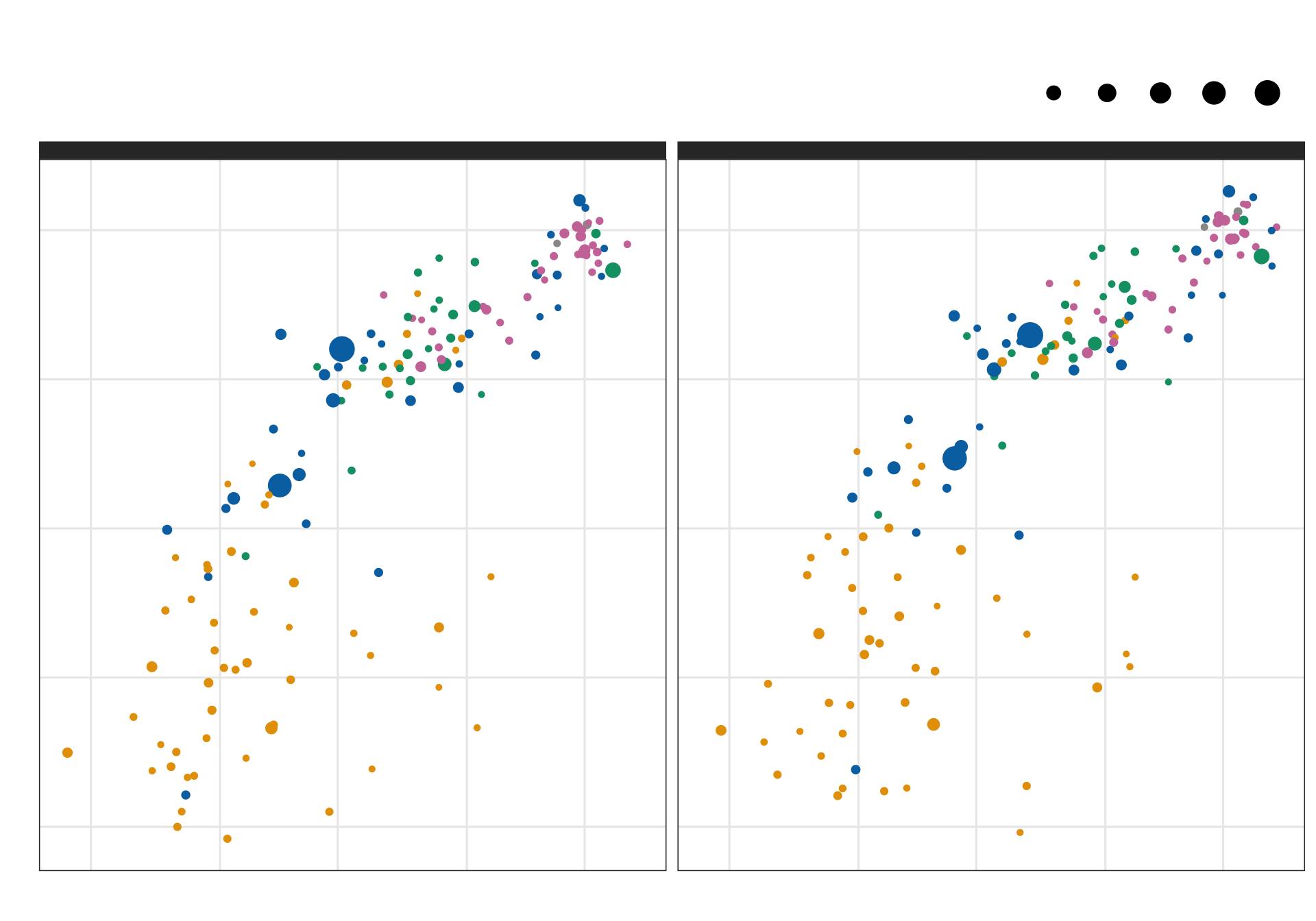
plot_nice
We can add some annotations
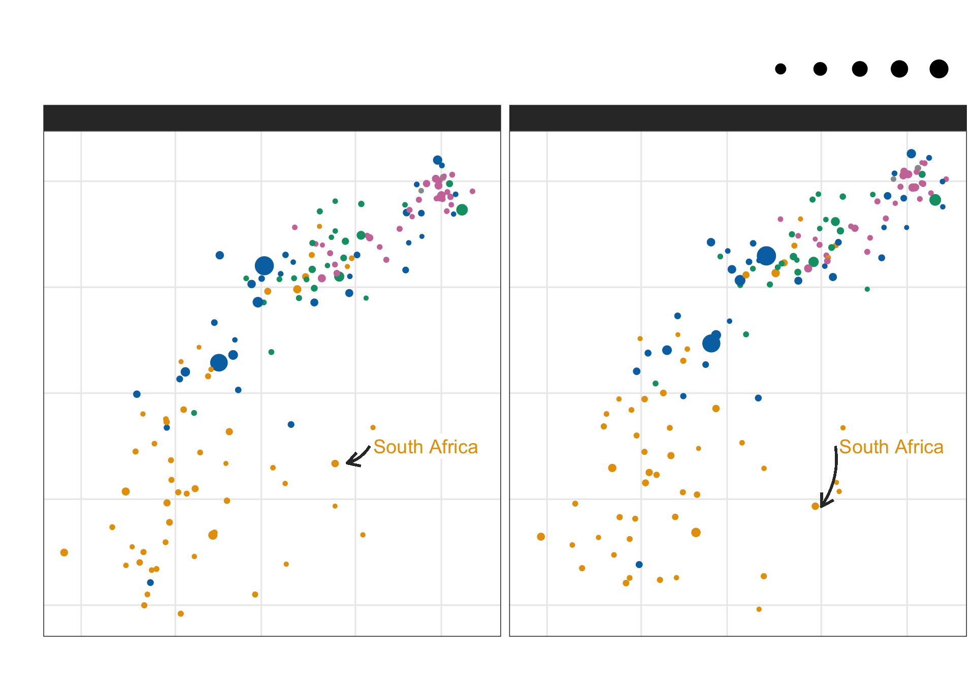
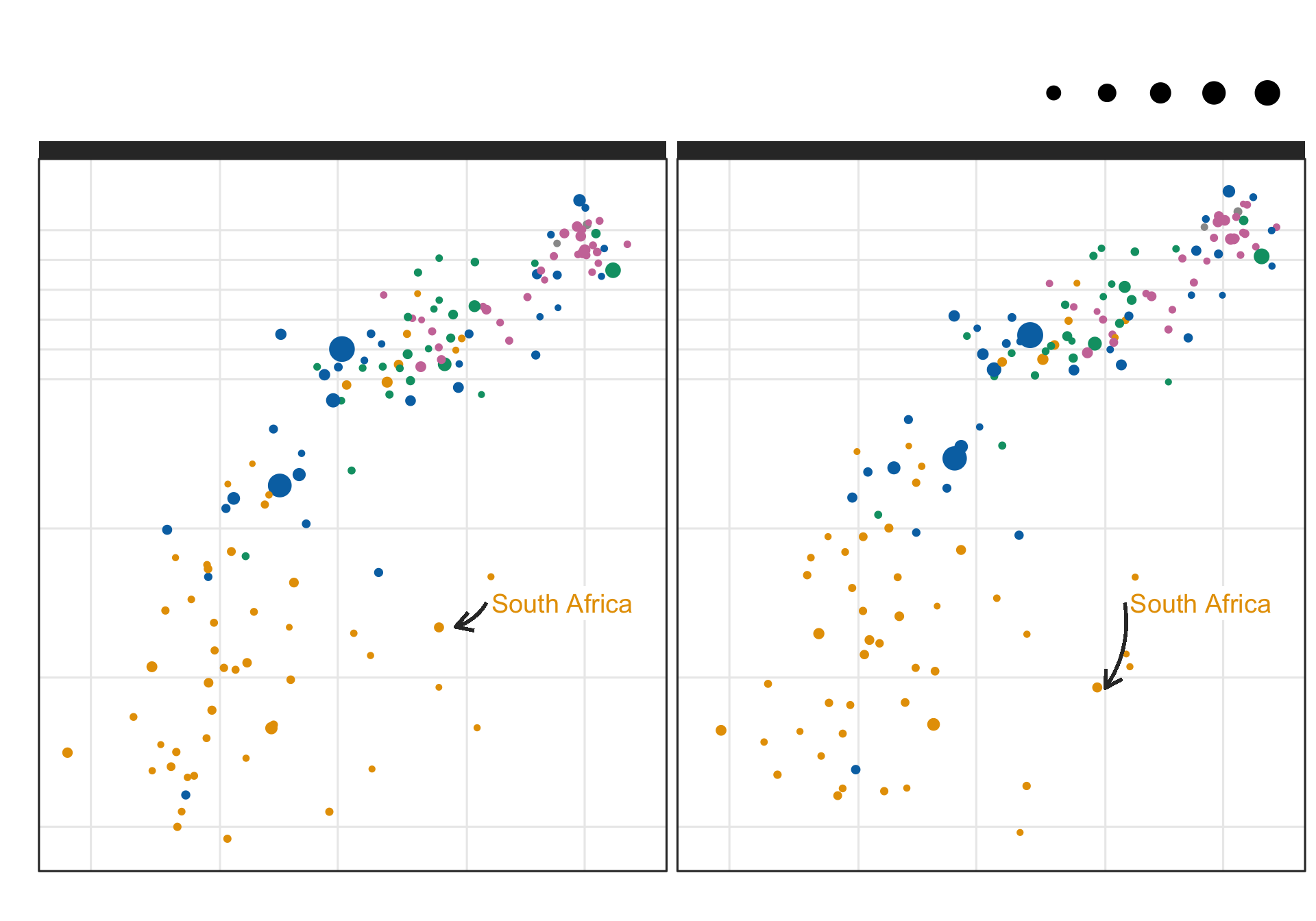
Annotionations can be great to highlight information that gets lost otherwise. For example we see that South Africa increases its GDP per capita from 2002 to 2007 but life expectancy decreases by 4 years.
#find african country with dip in lifeexp: South Africa(2002: x = 7711 ,y= 53.4; 2007: x = 9270, y = 49.3)
gapminder_filtered |>
  filter(continent == "Africa" & between(gdpPercap,3000,10000) & between(lifeExp,48,55)) |> arrange(desc(pop))
# A tibble: 6 × 6
  country           continent  year lifeExp      pop gdpPercap
  <fct>             <fct>     <int>   <dbl>    <int>     <dbl>
1 South Africa      Africa     2002    53.4 44433622     7711.
2 South Africa      Africa     2007    49.3 43997828     9270.
3 Congo, Rep.       Africa     2002    53.0  3328795     3484.
4 Namibia           Africa     2007    52.9  2055080     4811.
5 Namibia           Africa     2002    51.5  1972153     4072.
6 Equatorial Guinea Africa     2002    49.3   495627     7703.
Show code (39 lines)
# creat df for different arrow coordinations
df_2002 <-  gapminder_filtered %>%
  filter(year == 2002) %>%
  mutate(
    start_x = 12000,
    end_x = 9000,
    start_y = 55,
    end_y = 53.4
  )

# creat df for different arrow coordinations
df_2007 <-  gapminder_filtered %>%
  filter(year == 2007) %>%
  mutate(
    start_x = 12000,
    end_x = 10000,
    start_y = 55,
    end_y = 49.3
  )

plot_nice_anno <- plot_nice + geom_label(aes(x = 12000, y = 55, label = "South Africa"),
                  hjust = 0,
                  vjust = 0.5,
                  lineheight = 0.8,
                  colour = colors[1],
                  fill = "white",
                  label.size = NA,
                  size = 5)   +
  geom_curve(data = df_2002, aes(x = start_x, y = start_y, xend = end_x, yend = end_y),
             colour = "grey20",
             size=0.8,
             curvature = -0.2,
             arrow = arrow(length = unit(0.03, "npc"))) +
  geom_curve(data = df_2007, aes(x = start_x, y = start_y, xend = end_x, yend = end_y),
             colour = "grey20",
             size=0.8,
             curvature = -0.2,
             arrow = arrow(length = unit(0.03, "npc")))
plot_nice_anno
Lets keep playing around
plot_nice_anno +
  scale_y_continuous(
    breaks = c(4:7*10, seq(70, 80, by = 2))
    ) + coord_cartesian(clip = "off")
Back to top