Building a company theme for ggplot2

# Theme
tx_theme <- theme_minimal(base_size = 18) +
  theme(panel.grid.minor = element_blank(),
        panel.grid.major = element_line(color = "grey70",linetype = 1),
        # Bold, bigger title
        plot.title = element_text(face = "bold", size = rel(1.7), color = "#04d790"),
        # Plain, slightly bigger subtitle that is grey
        plot.subtitle = element_text(face = "plain", size = rel(1.3), color = "grey70"),
        # Italic, smaller, grey caption that is left-aligned
        plot.caption = element_text(face = "italic", size = rel(0.7),
                                    color = "grey70", hjust = 0),
        # Title left
        plot.title.position = "plot",
        # Bold legend titles
        legend.title = element_text(face = "bold"),
        # Bold, slightly larger facet titles that are left-aligned for the sake of repetition
        #strip.text = element_text(face = "bold", size = rel(1.1), hjust = 0),
        # Bold axis titles
        axis.title = element_text(face = "bold", color = "White"),
        # Tex color
        axis.text = element_text(color = "grey70"),
        # Add some space above the x-axis title and make it left-aligned
        axis.title.x = element_text(margin = margin(t = 15), hjust = 0),
        # Add some space to the right of the y-axis title and make it top-aligned
        axis.title.y = element_text(margin = margin(r = 15), hjust = 1),
        # Add a light grey background to the facet titles, with no borders
        #strip.background = element_rect(fill = "grey90", color = NA),
        # Add a thin grey border around all the plots to tie in the facet titles
        #panel.border = element_rect(color = "grey90", fill = NA),
        # Add color TX
        plot.background = element_rect(fill = color_tx[2]),
        plot.margin = margin(rep(18, 4)))



# plot Scatter
p <- ggplot(cars, aes(dist, speed)) +
  geom_point(color = "#04d790", size = 2) +
  labs(
    title = "Test, here goes title",
    x = "Distance",
    y = "Speed",
    subtitle = "Subtitle",
    caption = "Data:  Test data") +
  scale_x_continuous(limits = c(-5,125))  +
  tx_theme

# plot Bar
cars <- cars %>% mutate(fast = factor(ifelse(speed > median(speed), 1,0)))
p <- ggplot(cars, aes(fast,dist)) +
  geom_col(fill = color_tx[1]) +
  scale_x_discrete(labels=c('Slow', 'Fast'))+
  tx_theme

# Plot uncertainty

p <- ggplot(cars, aes(fast,dist)) +
  geom_boxplot(fill = color_tx[1]) +
  scale_x_discrete(labels=c('Slow', 'Fast'))+
  tx_theme

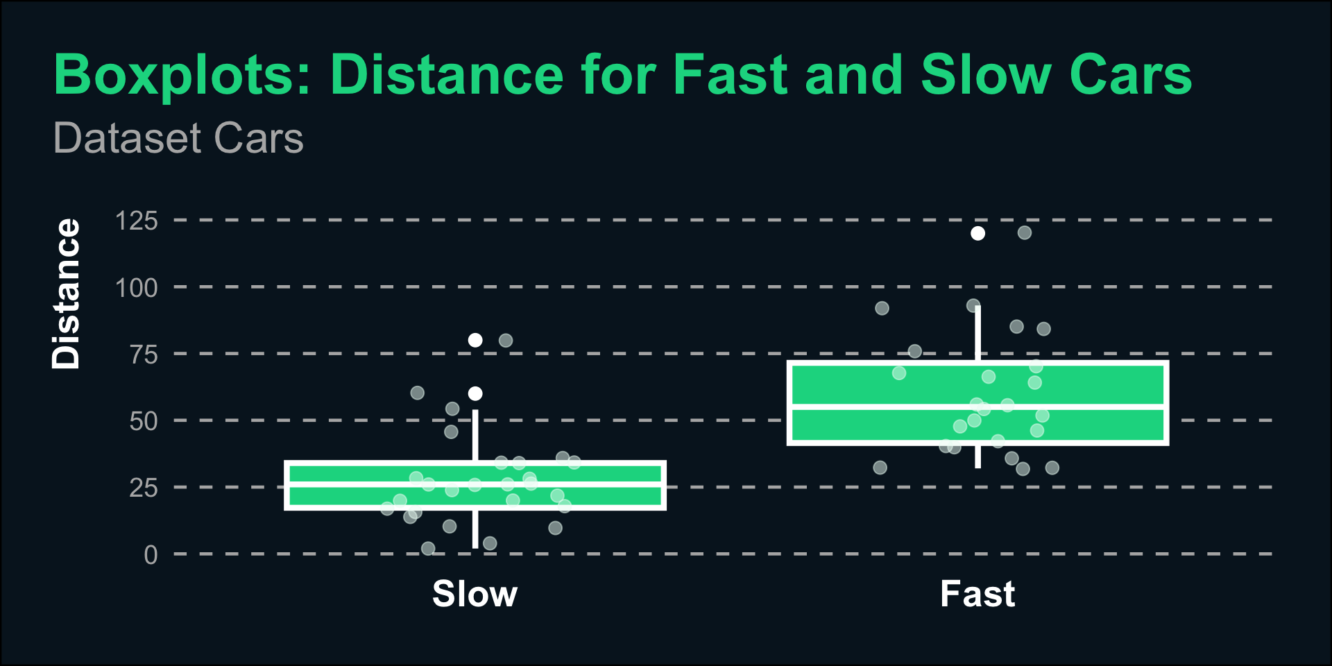
p <- ggplot(cars, aes(fast,dist)) +
  geom_boxplot(col = "white", fill = color_tx[1], linewidth = 1.5, fatten = 1, outlier.size = 3) +
  scale_x_discrete(labels=c('Slow', 'Fast'))+
  ## use either geom_point() or geom_jitter()
  geom_point(
    size = 3,
    alpha = .5,
    color = color_tx[3],
    position = position_jitter(
      ## control randomness and range of jitter
      seed = 1, width = .2
    ))   +
  labs(
    title = "Boxplots: Distance for Fast and Slow Cars",
    subtitle = "Dataset Cars",
    y = "Distance"
  ) +
  tx_theme +
  theme(panel.grid.major = element_line(linetype = 2),
                            panel.grid.major.x = element_blank(),
        axis.title.x = element_blank(),
        axis.text.x = element_text(face = "bold", size = 20, color = "white" ),
        axis.title.y = element_text(size = 20),
        plot.margin=unit(c(1,1,1,1), 'cm'),
        plot.subtitle = element_text(margin=margin(0,0,30,0)))

p